Swift is Now Fully Operational

The Swift satellite’s Ultraviolet/Optical Telescope (UVOT) has seen first light, capturing an image of the Pinwheel Galaxy, long loved by amateur astronomers as the “perfect” face-on spiral galaxy. The UVOT now remains poised to observe its first gamma-ray burst and the Swift observatory, launched into Earth orbit in November 2004, is now fully operational.

Swift is a NASA-led mission dedicated to the gamma-ray burst mystery. These random and fleeting explosions likely signal the birth of black holes. With the UVOT turned on, Swift now is fully operational. Swift’s two other instruments — the Burst Alert Telescope (BAT) and the X-ray Telescope (XRT) — were turned on over the past several weeks and have been snapping up gamma-ray bursts ever since.

“After many years of effort building the UVOT, it was exciting to point it toward the famous Pinwheel Galaxy, M101,” said Peter Roming, UVOT Lead Scientist at Penn State. “The ultraviolet wavelengths in particular reveal regions of star formation in the galaxy’s wispy spiral arms. But more than a pretty image, this first-light observation is a test of the UVOT’s capabilities.”

Swift’s three telescopes work in unison. The BAT detects gamma-ray bursts and autonomously turns the satellite in seconds to bring the burst within view of the XRT and the UVOT, which provide detailed follow-up observations of the burst afterglow. Although the burst itself is gone within seconds, scientists can study the afterglow for clues about the origin and nature of the burst, much like detectives at a crime scene.

The UVOT serves several important functions. First, it will pinpoint the gamma-ray burst location a few minutes after the BAT detection. The XRT provides a burst position within a 1- to-2-arcsecond range. The UVOT will provide sub-arcsecond precision, a spot on the sky far smaller than the eye of a needle at arm’s length. This information is then relayed to scientists at observatories around the world so that they can view the afterglow with other telescopes.

As the name applies, the UVOT captures the optical and ultraviolet component of the fading burst afterglow. “The ‘big gun’ optical observatories such as Hubble, Keck, and VLT have provided useful data over the years, but only for the later portion of the afterglow,” said Keith Mason, the U.K. UVOT Lead at University College London?s Mullard Space Science Laboratory. “The UVOT isn’t as powerful as these observatories, but has the advantage of observing from the very dark skies of space. Moreover, it will start observing the burst afterglow within minutes, as opposed to the day-long or week-long lag times inherent with heavily used observatories. The bulk of the afterglow fades within hours.”

The ultraviolet portion will be particularly revealing, said Roming. “We know nearly nothing about the ultraviolet part of a gamma-ray burst afterglow,” he said. “This is because the atmosphere blocks most ultraviolet rays from reaching telescopes on Earth, and there have been few ultraviolet telescopes in orbit. We simply haven’t yet reached a burst fast enough with a UV telescope.”

The UVOT’s imaging capability will enable scientists to understand the shape of the afterglow as it evolves and fades. The telescope’s spectral capability will enable detailed analysis of the dynamics of the afterglow, such as the temperature, velocity, and direction of material ejected in the explosion.

The UVOT also will help scientists determine the distance to the closer gamma-ray bursts, within a redshift of 4, which corresponds to a distance of about 11 billion light years. The XRT will determine distances to more distant bursts.

Scientists hope to use the UVOT and XRT to observe the afterglow of short bursts, less than two seconds long. Such afterglows have not yet been seen; it is not clear if they fade fast or simply don’t exist. Some scientists think there are at least two kinds of gamma-ray bursts: longer ones (more than two seconds) that generate afterglows and that seem to be caused by massive star explosions, and shorter ones that may be caused by mergers of black holes or neutron stars. The UVOT and XRT will help to rule out various theories and scenarios.

The UVOT is a 30-centimeter telescope with intensified CCD detectors and is similar to an instrument on the European Space Agency’s XMM-Newton mission. The UVOT is as sensitive as a four-meter optical ground-based telescope. The UVOT’s day-to-day observations, however, will look nothing like M101. Distant and faint gamma-ray burst afterglows will appear as tiny smudges of light even to the powerful UVOT. The UVOT is a joint product of Penn State and the Mullard Space Science Laboratory.

Swift is a medium-class explorer mission managed by NASA Goddard. Swift is a NASA mission with participation of the Italian Space Agency and the Particle Physics and Astronomy Research Council in the United Kingdom. It was built in collaboration with national laboratories, universities and international partners, including Penn State University in Pennsylvania, U.S.A.; Los Alamos National Laboratory in New Mexico, U.S.A.; Sonoma State University in California, U.S.A.; the University of Leicester in Leicester, England; the Mullard Space Science Laboratory in Dorking, England; the Brera Observatory of the University of Milan in Italy; and the ASI Science Data Center in Rome, Italy.

Original Source: Eberly College of Science News Release

Digging on Mars Won’t Be Easy

Imagine this scenario. The year is 2030 or thereabouts. After voyaging six months from Earth, you and several other astronauts are the first humans on Mars. You’re standing on an alien world, dusty red dirt beneath your feet, looking around at a bunch of mining equipment deposited by previous robotic landers.

Echoing in your ears are the final words from mission control: “Your mission, should you care to accept it, is to return to Earth–if possible using fuel and oxygen you mine from the sands of Mars. Good luck!”

It sounds simple enough, mining raw materials from a rocky, sandy planet. We do it here on Earth, why not on Mars, too? But it’s not as simple as it sounds. Nothing about granular physics ever is.

Granular physics is the science of grains, everything from kernels of corn to grains of sand to grounds of coffee. These are common everyday substances, but they can be vexingly difficult to predict. One moment they behave like solids, the next like liquids. Consider a dump truck full of gravel. When the truck begins to tilt, the gravel remains in a solid pile, until at a certain angle it suddenly becomes a thundering river of rock.

Understanding granular physics is essential for designing industrial machinery to handle vast quantities of small solids–like fine Martian sand.

The problem is, even here on Earth “industrial plants don’t work very well because we don’t understand equations for granular materials as well as we understand the equations for liquids and gases,” says James T. Jenkins, professor of theoretical and applied mechanics at Cornell University in Ithaca, N.Y. “That’s why coal-fired power plants operate at low efficiencies and have higher failure rates compared to liquid-fuel or gas-fired power plants.”

So “do we understand granular processing well enough to do it on Mars?” he asks.

Let’s start with excavation: “If you dig a trench on Mars, how steep can the sides be and remain stable without caving in?” wonders Stein Sture, professor of civil, environmental, and architectural engineering and associate dean at the University of Colorado in Boulder. There’s no definite answer, not yet. The layering of dusty soils and rock on Mars isn’t well enough known.

Some information about the mechanical composition of the top meter or so of Martian soils could be gained by ground-penetrating radar or other sounding devices, Sture points out, but much deeper and you “probably need to take core samples.” NASA’s Phoenix Mars lander (landing 2008) will be able to dig trenches about a half-meter deep; the 2009 Mars Science Laboratory will be able to cut out rock cores. Both missions will provide valuable new data.

To go even deeper, Sture (in connection with the University of Colorado’s Center for Space Construction) is developing innovative diggers whose business ends vibrate into soils. Agitation helps break cohesive bonds holding compacted soils together and can also help mitigate the risk of soils collapsing. Machines like these might one day go to Mars, too.

Another problem is “hoppers”–the funnels miners use to guide sand and gravel onto conveyor belts for processing. Knowledge of Martian soils would be vital in designing the most efficient and maintenance-free hoppers. “We don’t understand why hoppers jam,” Jenkins says. Jams are so frequent, in fact, that “on Earth, every hopper has a hammer close by.” Banging on the hopper frees the jam. On Mars, where there would be only a few people around to tend equipment, you’d want hoppers to work better than that. Jenkins and colleagues are researching why granular flows jam.

And then there’s transportation: The Mars rovers Spirit and Opportunity have had little trouble driving miles around their landing sites since 2004. But these rovers are only about the size of an average office desk and only about as massive as an adult. They’re go-carts compared to the massive vehicles possibly needed for transporting tons of Martian sand and rock. Bigger vehicles are going to have a tougher time getting around.

Sture explains: As early as the 1960s when scientists were first studying possible solar-powered rovers for negotiating loose sands on the Moon and other planets, they calculated “that the maximum viable continuous pressure for rolling contact pressure over Martian soils is only 0.2 pounds per square inch (psi),” especially when traveling up or down slopes. This low figure has been confirmed by the behavior of Spirit and Opportunity.

A rolling contact pressure of only 0.2 psi “means that a vehicle has to be light-weight or has to have a way of effectively distributing the load to many wheels or tracks. Reducing contact pressure is crucial so the wheels don’t dig into soft soil or break through duricrusts [thin sheets of cemented soils, like the thin crust on windblown snow on Earth] and get stuck.”

That requirement implies that a vehicle for moving heavier loads–people, habitats, equipment–might be “a huge Fellini-type thing with wheels 4 to 6 meters (12 to 18 feet) in diameter,” says Sture, referring to the famous Italian director of surreal films. Or it might have enormous open-mesh metal treads like a cross between highway-construction backhoes on Earth and the lunar rover used during the Apollo program on the Moon. Thus, tracked or belted vehicles seem promising for carrying large payloads.

A final challenge facing granular physicists is to figure out how to keep equipment operating through Mars’ seasonal dust storms. Martian storms whip fine dust through the air at velocities of 50 m/s (100+ mph), scouring every exposed surface, sifting into every crevice, burying exposed structures both natural and manmade, and reducing visibility to meters or less. Jenkins and other investigators are studying the physics of aeolian [wind] transporting of sand and dust on Earth, both to understand the formation and moving of dunes on Mars, and also to ascertain what sites for eventual habitats might be best protected from prevailing winds (for example, in the lee of large rocks).

Returning to Jenkins’s big question, “do we understand granular processing well enough to do it on Mars?” The unsettling answer is: we don’t yet know.

Working with imperfect knowledge is okay on Earth because, usually, no one suffers much from that ignorance. But on Mars, ignorance could mean reduced efficiency or worse preventing the astronauts from mining enough oxygen and hydrogen to breathe or use for fuel to return to Earth.

Granular physicists analyzing data from the Mars rovers, building new digging machines, tinkering with equations, are doing their level best to find the answers. It’s all part of NASA’s strategy to learn how to get to Mars … and back again.

Original Source: Science@NASA

Interview Asteroid Researcher Dr. David J. Tholen

With all the recent news about asteroids and comets, I figure you’ve got a lot of questions. Well, now’s your chance to get some answers. We’ve lined up astronomer Dr. David J. Tholen, a professor at the University of Hawaii, Institute for Astronomy who specializes in the search for Earth-crossing asteroids. Once again, visit the forum, post your questions for David, and we’ll pick through and send him some zingers. I’ll publish his answers in an upcoming issue of Universe Today.

Click here to visit the forum and post your question.

Thanks!

Fraser Cain
Publisher
Universe Today

What’s Up This Week – Jan 31 – Feb 6, 2005

Image credit: Emmanuel Mallart
Monday, January 31 – So, where is Comet Machholz and what has it been doing while the Moon was out? Heading north! As we’ve watched its rapid progress (a degree a day at times!) since it first appeared in the south, you will now find Machholz tonight just southeast of Eta Cassiopeia. Having made its closest approach to the Sun and heading for the outer limits, C/2004 Q2 will soon start to shrink and fade, but it’s still a prime time player! Catch it tonight…

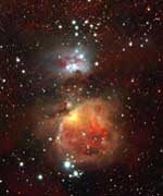
As we relaxed and viewed the “Great Orion Nebula” last week, I am sure that many of you realize this is a highly complex region of sky that deserves much more attention to detail. With the Moon satisfactorily out of the way during the early evening hours, let’s take the time to do a much more serious study over the next few evenings.

Tonight our goal is Iota Orionis. Known to the Arabs as “the Bright One of the Sword”, we know it as the southern-most star in its asterism’s namesake. Iota is estimated to be around 2000 light years away and is about 20,000 times brighter than our own Sol, but in the telescope you will find Iota to be an easy and charming triple star. The bluish B star is relatively close at 11″ in separation, but a bright 6.9 in magnitude. Much more distant at 50″ is the reddish C star, and far more disparate at magnitude 11. Iota itself is a spectroscopic binary and you will note another “white” double (Struve 747) unrelated to Iota about 8′ to the southwest.

Staying at high power, the reason I ask you to look here tonight is not to conquer a Herschel 400 object, but to study a region of the sky that would be far more impressive if it weren’t for its alluring neighbor. If you look closely, you will see that Iota is involved in a great region of emission nebula known as the NGC 1900 along with a small open cluster known as H 31. To be sure, the area is vague, as are all low surface brightness nebulae, but do look to the east of Iota where a much brighter, roundish area makes an unmistakable appearance!

Tuesday, February 1 – If you are up early this morning, today is the best time to catch lunar feature – Rupes Recta. The angle of the lighting will be just perfect to highlight this 110 km long feature!

Please take a moment to remember Columbia – the first Space Shuttle to travel to Earth orbit – and its brave crew who left us two years ago today. Rick D. Husband, William C. McCool, Michael P. Anderson, David M. Brown, Kalpana Chawla, Laurel Blair Salton Clark, and Ilan Ramon… We wish you godspeed.

Tonight let’s head for the “holy grail” of multiple star systems as we look into the fueling core of the M42 – Theta Orionis. Are you ready to walk into “the Trap”? Even the smallest of telescopes can reveal the four bright stars that comprise the quadrangle at the heart of the Great Orion Nebula known as the “Trapezium”. Both the beginner and the seasoned veteran know that there are actually eight stars in this region and the journey we are about to undertake requires both aperture and fine skies. But what can you really see?

All four primary stars are easy. A steady hand with binoculars and even the most modest of telescopes make this foursome an awesome sight… And they seem to be in a dark “notch” of their own, don’t they? A telescope of 150mm in aperture will reveal two additional 11th magnitude stars, but excellent skies could mean the even smaller aperture could detect them. They will appear as “red” companions to the “blue/white” primary stars. But what of the other two? The remaining two components average about magnitude 16, putting them within reach of large amateur scopes, but what would you see?

When I first began observing the Trapezium area with a 12.5″ telescope, I was sure that I would never see the two faintest members of the group. I was new to challenging double stars and had never looked at a diagram. (To this day, I still prefer to observe and describe things first and confirm them later. Knowing in advance what you are “supposed” to see colours what you “can” see.) I had seen the fainter stars that appeared as doubles, along with a faint wink here and there as well as one to the outside that made the whole thing appear like a pentagon. Little did I realize I was perceiving all eight members, and there seemed to be so much more just on the edge of my perception. Thus began my own personal quest to study the “Trapezium” on a more professional level, just like challenging galaxy studies.

Using the 31″ reflector at Warren Rupp Observatory, it was time to “walk into the Trap” and to answer all my observing questions through visual confirmation. While at first glance with a small telescope, the background region in this area might appear a black void – it is not. The nebula continues here, but changes form. Instead of seeing “smoke-like” filaments, the region around the Trapezium is scalloped, like fish scales. You can never see this in a photograph! I realized immediately that both the G and H stars that I had always questioned were quite within range of my 12.5″ as I recognized the pattern. Then a moment of perfect clarity came and the view literally exploded in dozens of stars buried within the field surrounding these eight known as the “Trapezium”.

Upon formal study, I found that there are around 300 such stars within 5′ of the Theta Orionis complex that exceed magnitude 17. According to Strand, the expansion rate puts them at an approximate age of 30,000 years, making it the youngest star cluster known. Regardless of what size telescope you use, you owe it to yourself to take the time to power up on the “Trap”. Since the time the area was revealed to my eyes in all its open glory, I have seen scallops in the nebula and both fainter members on nights with exceptional seeing in much smaller telescopes. No matter how many stars you are able to resolve out of this region, you are looking into the very beginnings of starbirth… A womb with a view!

Wednesday, February 2 – Do you get up for work before dawn? Take a moment to step outside and have a look at Jupiter. Our solar system’s largest planet will go stationary (retro) in its orbit during the early morning hours. You’ll find it within 3 degrees of Spica!

Tonight our study region is to the northeast of the Great Orion Nebula (M42) and has a designation of its own – M43. Discovered by De Mairan in the latter half of the 18th century, this emission nebula appears to be separate from the M42, but the division known as “the Fish Mouth” is actually caused by dark gas and dust within the nebula itself. At the heart of it is 7th magnitude “Bond’s Star” – and wouldn’t 007 be proud? This unusually bright OB star is creating a matter-bound Stromgren sphere!

Translated loosely, this star is actually ionizing the gas near it, making a orb shaped area of glowing hydrogen gas. Its size is governed by the density of both the gas and dust that surround “Bond’s Star”. This “exciting” star of our show is more properly known as Nu Orionis and near it lies a dense concentration of neutral material known as the “Orion Ridge”. It is this combination of dust – mixed with gases – that make for a well balanced area of star formation!

And besides… It’s just cool. 😉

Thursday, February 3 – This morning at 14:00 UT, the Moon will have reached maximum libration, turning Crater Otto Struve our way. And speaking of the Moon, on this day in 1966, the first soft landing on the lunar surface was achieved by Soviet Luna 9. Spaseba!

Lace up your Nikes and let’s head out tonight above The Great Orion Nebula and find “The Running Man”…

Located just a half a degree north of the M43, this tripartite nebula consists of three separate areas of emission and reflection nebulae that seem to be visually connected. The NGC 1977, NGC 1975 and NGC1973 would probably be pretty spectacular if they were a bit more distant from their grand neighbor! This whispery soft, conjoining nebula’s fueling source is multiple star 42 Orionis. To the eye, a lovely “triangle” of bright nebula with several enshrouded stars make a wonderfully large region for exploration. Can you see the “Running Man” within?

Friday, February 4 – Wake up, Europe! This morning the crescent Moon will occult Antares for a substantial portion of viewers. Please check IOTA tables for viewing areas and times. Klare nacht!

For those of us not so fortunate, we can always look about 8 degrees north of Mars this morning for Pluto as we note its discoverer – Clyde Tombaugh – born on this day in 1906.

Let’s return again to Orion tonight, but preferably with binoculars since we will be studying a very large region known as “Barnard’s Loop”. Extending in a massive area about the size of the “bow”, you will find Barnard’s photographic namesake to the eastern edge of Orion, where it extends almost half the size of the constellation between Alpha and Kappa.

Because the Orion complex contains so many rapidly evolving stars, it stands to reason that a supernova should have occurred at some time. “Barnard’s Loop” is quite probably the shell leftover from such a cataclysmic event. If taken as a “whole”, it would encompass 10 degrees of sky!

For the most past, the nebula itself is very vague, but the eastern arc (where we are observing tonight) is relatively well defined against the starry field. Although it is similar to the Cygus Loop (“Veil Nebula”), our Barnard Loop is far more ancient. If you have transparent, dark skies? Enjoy! You can trace several degrees of this ancient remnant using just binoculars.

Saturday, February 5 – On this day in 1963, the first quasar redshift was measured by Maarten Schmidt and in 1974 Mariner 10 captured the first close-up photos of Venus.

Tonight I ask you to once again take out your telescopes and explore a region with me that we have previously visited – the M78. It is for the very sake of amateur astronomy that I ask you to do this… And here is why!

On January 23, 2004 a young backyard astronomer named Jay McNeil was checking out his new 3″ telescope by taking some long exposures of the M78. Little did Jay know at the time, but he was about to make a huge discovery! When he later developed his photographs, there was a nebulous patch there that had no designation. When he reported his findings to the professionals, they confirmed it had no official designation and that Jay had stumbled onto something quite unique! It is believed that Jay’s discovery was a variable accretion disc around newborn star – IRAS 05436-0007. Little is known about the region, but it seems that it had been caught in a photo once in the past but never studied. Even the Digital Sky Surveys had no record of it!

Although Jay’s discovery might not be bright enough tonight to be seen just south of the M78, it is a variable and circumstance plays a big role in any observation. Before you think that being a backyard astronomer has no real importance to science — remember a teenager in a Kentucky backyard with a 3″ telescope…

Catching what professionals had missed!

Sunday, February 6 – Do you need a smile? Then look at the waning crescent Moon this morning. On this day in 1971, Apollo 14 astronaut Alan Shepherd was the first human to “tee off” from the lunar surface! I wonder if that golf ball is still orbiting?!

Tonight let’s return again to Orion’s “Belt” and bright eastern star Zeta. Having visited this before, we know Alnitak is a delightful triple as well as home to the incredible “Flame” and “Horsehead” nebula. Heading next to the western-most of the trio, we find Delta – or Mintaka. Even small telescopes will be delighted to find that Mintaka is also a double with its 6.7 magnitude “blue” companion at an easy separation of 53″ north of the primary.

But you knew I was saving the best for last, didn’t you?

Now let’s go for the center-most star and identify Epsilon. Known to the Arabs as Alnilam, or the “Belt of Pearls”, Epsilon is a super-giant star that resides about 1600 light years away from us. For those with average telescopes, you will notice a “haze” around Alnilam and you would be correct. It is also surrounded by a reflection nebula
NGC1990 – a circular gaseous region that spans around 20 light years, fueled by Epsilon’s bluish light. The NGC1990 is surrounded by “Herbig-Haro” or “HH” bi-polar jets. It is rumored that an 8″ or 10″ telescope at 250x will reveal these globules as 14th magnitude “fuzzy stars”. What do you see?

Until next week? Keep exploring the fantastic Orion region. There are many planetary nebulae and open star clusters (even a galaxy or two) waiting for you! Do not be discouraged if you cannot see some of these things on your first try – astronomy is like anything else – it takes Practice! If you don’t have skies tonight? Have Patience. And if you are still learning what type of conditions it takes to see things at their best? Be Persistent! Practice + Patience + Persistence = Perfection!

Light speed…. ~Tammy Plotner

Mars Glows at Night

Image credit: ESA
The SPICAM instrument on board ESA?s Mars Express has detected light emissions over the nightside of Mars caused by the production of nitrogen oxide in the atmosphere.

SPICAM is a dual ultraviolet/infrared spectrometer dedicated primarily to the study of the atmosphere and ionosphere of Mars. Spectroscopy of ?airglow? and radiometry are powerful methods for remote sensing investigations of the physics of upper atmospheres of the terrestrial planets.

For instance, Martian ?dayglow? spectra reveal the effect of extreme ultraviolet radiation from the Sun on carbon dioxide in Mars?s upper atmosphere, and show it to be a major heating mechanism and involved in the production of an ionosphere.

?Dayglow? and ?nightglow? effects are emissions of light in the upper atmosphere which are produced when atoms combine to form molecules, releasing energy in the form of photons. Dayglow is visible in the dayside upper atmosphere, and nightglow over the nightside.

The ultraviolet spectrum of the nightglow seen by SPICAM is produced when nitrogen and oxygen atoms combine to produce nitrogen oxide molecules (?recombination?) and release energy.

A similar ultraviolet nightglow on Venus had been detected with Mariner 5 and Pioneer Venus, but the first real evidence for this process was a spectrum acquired with the ESA/NASA International Ultraviolet Explorer satellite which identified the nightglow emissions as coming from nitrogen oxide recombination.

Scientists proposed that nitrogen and oxygen atoms are produced on the Venus day side by a process called ?electron ultraviolet photodissociation?. This is the break-up of oxygen, nitrogen and carbon dioxide molecules by ultraviolet light. The separate atoms were then transported to the nightside where recombination occurs.

These findings were later supported by detailed Pioneer Venus spectra and computer modelling of Venusian atmospheric circulation. Until now, however, this kind of nightglow had never been seen on Mars. It is thought that the mechanism responsible for the nightglow emissions on Mars is the same as that causing the nightglow on Venus.

These nightglow emissions are important tracers of atmospheric transport at high altitudes, which could be used in refining circulation models of the Martian atmosphere.

Original Source: ESA News Release

Pluto and Charon Could Have Formed Together

The evolution of Kuiper Belt objects, Pluto and its lone moon Charon may have something in common with Earth and our single Moon: a giant impact in the distant past.

Dr. Robin Canup, assistant director of Southwest Research Institute’s? (SwRI) Department of Space Studies, argues for such an origin for the Pluto-Charon pair in an article for the January 28 issue of the journal Science.

Canup, who currently is a visiting professor at the California Institute of Technology, has worked extensively on a similar “giant collision” scenario to explain the Moon’s origin.

In both the Earth-Moon and Pluto-Charon cases, Canup’s smooth particle hydrodynamic simulations depict an origin in which a large, oblique collision with the growing planet produced its satellite and provided the current planet-moon system with its angular momentum.

While the Moon has only about 1 percent of the mass of Earth, Charon accounts for a much larger 10 to 15 percent of Pluto’s total mass. Canup’s simulations suggest that a proportionally much larger impactor – one nearly as large as Pluto itself – was responsible for Charon, and that the satellite likely formed intact as a direct result of the collision.

According to Canup, a collision in the early Kuiper Belt – a disk of comet-like objects orbiting in the outer solar system beyond Neptune – could have given rise to a planet and satellite with relative sizes and angular rotation characteristics consistent with those of the Pluto-Charon pair. The colliding objects would have been about 1,600 to 2,000 kilometers in diameter, or each about half the size of the Earth’s Moon.

“This work suggests that despite their many differences, our Earth and the tiny, distant Pluto may share a key element in their formation histories. This provides further support for the emerging view that stochastic impact events may have played an important role in shaping final planetary properties in the early solar system,” said Canup.

The “giant impact” theory was first proposed in the mid-1970s to explain how the Moon formed, and a similar mode of origin was suggested for Pluto and Charon in the early 1980s. Canup’s simulations are the first to successfully model such an event for the Pluto-Charon pair.

Simulations published by Canup and a colleague in Nature in 2001 showed that a single impact by a Mars-sized object in the late stages of Earth’s formation could account for the iron-depleted Moon and the masses and angular momentum of the Earth-Moon system.

This was the first model to simultaneously explain these characteristics without requiring that the Earth-Moon system be substantially modified after the lunar forming impact.

This research was supported by the National Science Foundation under grant no. AST0307933.

Original Source: SwRI News Release

Keep an Eye on the Weather in Space

NASA is returning to the Moon–not just robots, but people. In the decades ahead we can expect to see habitats, greenhouses and power stations up there. Astronauts will be out among the moondust and craters, exploring, prospecting, building.

Good thing.

On January 20th, 2005, a giant sunspot named “NOAA 720” exploded. The blast sparked an X-class solar flare, the most powerful kind, and hurled a billion-ton cloud of electrified gas (a “coronal mass ejection”) into space. Solar protons accelerated to nearly light speed by the explosion reached the Earth-Moon system minutes after the flare–the beginning of a days-long “proton storm.”

Here on Earth, no one suffered. Our planet’s thick atmosphere and magnetic field protects us from protons and other forms of solar radiation. In fact, the storm was good. When the plodding coronal mass ejection arrived 36 hours later and hit Earth’s magnetic field, sky watchers in Europe saw the brightest and prettiest auroras in years: gallery.

The Moon is a different story.

“The Moon is totally exposed to solar flares,” explains solar physicist David Hathaway of the Marshall Space Flight Center. “It has no atmosphere or magnetic field to deflect radiation.” Protons rushing at the Moon simply hit the ground–or whoever might be walking around outside.

The Jan. 20th proton storm was by some measures the biggest since 1989. It was particularly rich in high-speed protons packing more than 100 million electron volts (100 MeV) of energy. Such protons can burrow through 11 centimeters of water. A thin-skinned spacesuit would have offered little resistance.

“An astronaut caught outside when the storm hit would’ve gotten sick,” says Francis Cucinotta, NASA’s radiation health officer at the Johnson Space Center. At first, he’d feel fine, but a few days later symptoms of radiation sickness would appear: vomiting, fatigue, low blood counts. These symptoms might persist for days.

Astronauts on the International Space Station (ISS), by the way, were safe. The ISS is heavily shielded, plus the station orbits Earth inside our planet’s protective magnetic field. “The crew probably absorbed no more than 1 rem,” says Cucinotta.

One rem, short for Roentgen Equivalent Man, is the radiation dose that causes the same injury to human tissue as 1 roentgen of x-rays. A typical dental x-ray, for example, delivers about 0.1 rem. So, for the crew of the ISS, the Jan. 20th proton storm was like 10 trips to the dentist–scary, but no harm done.

On the Moon, Cucinotta estimates, an astronaut protected by no more than a space suit would have absorbed about 50 rem of ionizing radiation. That’s enough to cause radiation sickness. “But it would not have been fatal,” he adds.

Right: The Jan. 20th proton storm photographed from space by a coronagraph onboard the Solar and Heliospheric Observatory (SOHO). The many speckles are solar protons striking the spacecraft’s digital camera. [More]

To die, you’d need to absorb, suddenly, 300 rem or more.

The key word is suddenly. You can get 300 rem spread out over a number of days or weeks with little effect. Spreading the dose gives the body time to repair and replace its own damaged cells. But if that 300 rem comes all at once … “we estimate that 50% of people exposed would die within 60 days without medical care,” says Cucinotta.

Such doses from a solar flare are possible. To wit: the legendary solar storm of August 1972.

It’s legendary (at NASA) because it happened during the Apollo program when astronauts were going back and forth to the Moon regularly. At the time, the crew of Apollo 16 had just returned to Earth in April while the crew of Apollo 17 was preparing for a moon-landing in December. Luckily, everyone was safely on Earth when the sun went haywire.

“A large sunspot appeared on August 2, 1972, and for the next 10 days it erupted again and again,” recalls Hathaway. The spate of explosions caused, “a proton storm much worse than the one we’ve just experienced,” adds Cucinotta. Researchers have been studying it ever since.

Cucinotta estimates that a moonwalker caught in the August 1972 storm might have absorbed 400 rem. Deadly? “Not necessarily,” he says. A quick trip back to Earth for medical care could have saved the hypothetical astronaut’s life.

Surely, though, no astronaut is going to walk around on the Moon when there’s a giant sunspot threatening to explode. “They’re going to stay inside their spaceship (or habitat),” says Cucinotta. An Apollo command module with its aluminum hull would have attenuated the 1972 storm from 400 rem to less than 35 rem at the astronaut’s blood-forming organs. That’s the difference between needing a bone marrow transplant ? or just a headache pill.

Modern spaceships are even safer. “We measure the shielding of our ships in units of areal density–or grams per centimeter-squared,” says Cucinotta. Big numbers, which represent thick hulls, are better:

The hull of an Apollo command module rated 7 to 8 g/cm2.

A modern space shuttle has 10 to 11 g/cm2.

The hull of the ISS, in its most heavily shielded areas, has 15 g/cm2.

Future moonbases will have storm shelters made of polyethelene and aluminum possibly exceeding 20 g/cm2.

A typical space suit, meanwhile, has only 0.25 g/cm2, offering little protection. “That’s why you want to be indoors when the proton storm hits,” says Cucinotta.

But the Moon beckons and when explorers get there they’re not going to want to stay indoors. A simple precaution: Like explorers on Earth, they can check the weather forecast–the space weather forecast. Are there any big ‘spots on the sun? What’s the chance of a proton storm? Is a coronal mass ejection coming?

All clear? It’s time to step out.

Original Source: Science@NASA Article

Biggest Stars Make the Biggest Magnets

Astronomy is a science of extremes–the biggest, the hottest, and the most massive. Today, astrophysicist Bryan Gaensler (Harvard-Smithsonian Center for Astrophysics) and colleagues announced that they have linked two of astronomy’s extremes, showing that some of the biggest stars in the cosmos become the strongest magnets when they die.

“The source of these very powerful magnetic objects has been a mystery since the first one was discovered in 1998. Now, we think we have solved that mystery,” says Gaensler.

The astronomers base their conclusions on data taken with CSIRO’s Australia Telescope Compact Array and Parkes radio telescope in eastern Australia.

A magnetar is an exotic kind of neutron star–a city-sized ball of neutrons created when a massive star’s core collapses at the end of its lifetime. A magnetar typically possesses a magnetic field more than one quadrillion times (one followed by 15 zeroes) stronger than the earth’s magnetic field. If a magnetar were located halfway to the moon, it could wipe the data from every credit card on earth.

Magnetars spit out bursts of high-energy X-rays or gamma rays. Normal pulsars emit beams of low-energy radio waves. Only about 10 magnetars are known, while astronomers have found more than 1500 pulsars.

“Both radio pulsars and magnetars tend to be found in the same regions of the Milky Way, in areas where stars have recently exploded as supernovae,” explains Gaensler. “The question has been: if they are located in similar places and are born in similar ways, then why are they so different?”

Previous research has hinted that the mass of the original, progenitor star might be the key. Recent papers by Eikenberry et al (2004) and Figer et al (2005) have suggested this connection, based on finding magnetars in clusters of massive stars.

“Astronomers used to think that really massive stars formed black holes when they died,” says Dr Simon Johnston (CSIRO Australia Telescope National Facility). “But in the past few years we’ve realized that some of these stars could form pulsars, because they go on a rapid weight-loss program before they explode as supernovae.”

These stars lose a lot of mass by blowing it off in winds that are like the sun’s solar wind, but much stronger. This loss would allow a very massive star to form a pulsar when it died.

To test this idea, Gaensler and his team investigated a magnetar called 1E 1048.1-5937, located approximately 9,000 light-years away in the constellation Carina. For clues about the original star, they studied the hydrogen gas lying around the magnetar, using data gathered by CSIRO’s Australia Telescope Compact Array radio telescope and its 64-m Parkes radio telescope.

By analyzing a map of neutral hydrogen gas, the team located a striking hole surrounding the magnetar. “The evidence points to this hole being a bubble carved out by the wind that flowed from the original star,” says Naomi McClure-Griffiths (CSIRO Australia Telescope National Facility), one of the researchers who made the map. The characteristics of the hole indicate that the progenitor star must have been about 30 to 40 times the mass of the sun.

Another clue to the pulsar/magnetar difference may lie in how fast neutron stars are spinning when they form. Gaensler and his team suggest that heavy stars will form neutron stars spinning at up to 500-1000 times per second. Such rapid rotation should power a dynamo and generate superstrong magnetic fields. `Normal’ neutron stars are born spinning at only 50-100 times per second, preventing the dynamo from working and leaving them with a magnetic field 1000 times weaker, says Gaensler.

“A magnetar goes through a cosmic extreme makeover and ends up very different from its less exotic radio pulsar cousins,” he says.

If magnetars are indeed born from massive stars, then one can predict what their birth rate should be, compared to that of radio pulsars.

“Magnetars are the rare `white tigers’ of stellar astrophysics,” says Gaensler. “We estimate that the magnetar birth rate will be only about a tenth that of normal pulsars. Since magnetars are also short-lived, the ten we have already discovered may be almost all that are out there to be found.”

The team’s result will be published in an upcoming issue of The Astrophysical Journal Letters.

This press release is being issued in conjunction with CSIRO’s Australia Telescope National Facility.

Headquartered in Cambridge, Mass., the Harvard-Smithsonian Center for Astrophysics (CfA) is a joint collaboration between the Smithsonian Astrophysical Observatory and the Harvard College Observatory. CfA scientists, organized into six research divisions, study the origin, evolution and ultimate fate of the universe.

Original Source: CfA News Release

Dr. Seth Shostak Answers Your Questions About SETI

Is there any other way a civilization can be detected other than by EM radiation (IR, UV, radiowave, microwave, etc) detection? What’s the probability of finding an intelligent lifeform in our lifetime? – Alfchemist

Well, sure, there are other possibilities for finding cosmic company. You could look for messages being transmitted by particle beams (even neutrinos), and this has been suggested. But the problem is that these require harder-to-build transmitters and receivers, and are also susceptible to absorption by interstellar gas. So they don’t seem to offer much advantage. The other possibility is to find some evidence of “alien engineering” — maybe sophisticated beings on other worlds have managed to rearrange the stars in their neighborhood, or build huge, starshine-collecting solar panels that we could somehow spot from afar. Some experiments have been done to locate such massive construction projects, but it’s hard to know how to look or even what to look for.

I think it’s likely that the new telescopes being built for SETI will trip across a signal by the year 2025.

The SETI Project and SETI@home have processed a bunch of data. Other than the search for intelligent signals, have you learned anything new about the universe from all this information? – corkft

In fact, not too much. This is rather surprising, because the history of astronomy suggests that whenever you build a new instrument, able to look at a previously unobserved bit of either space or the spectrum, you usually trip across some unexpected object or other. SETI projects have receivers with VERY narrow frequency channels. But there really doesn’t seem to be any natural phenomena that lend themselves to being discovered with such equipment. In a sense this justifies SETI’s assumption that any narrow-band signal would convincingly prove intelligence!

What is the maximum distance at which SETI can detect signals which are not deliberately beamed at us, such as normal radio telecommunications traffic? And are there plans to increase this range? – Steve t

Our best SETI experiments to date could detect Earth-like “leakage” signals at no more than 1 light-year’s distance. So not too far. But keep in mind that (1) our experiments do get more sensitive with time, so this distance will increase, and (2) we’ve only had radio for a century. Aliens, who may have invented this technology thousands or even millions of years ago, will undoubtedly have some transmitters and antenna systems capable of putting out signals far more powerful than what we manage with our erudite and always entertaining commercial television efforts!

To what degree does our SETI search make assumptions about the rate of information transfer? What transfer rates are we currently equipped to detect, and in what modulation modes? – wstevenbrown

We don’t worry at all about modulation, or schemes for encoding messages. That’s something to be considered after you’ve found that their transmitter is on! At the moment, all SETI experiments simply look for narrow-band (typically 1 Hz or narrower) components to a signal… somewhat akin to the “carrier” signal for earthly transmissions, but not limited to those. We also look for slowly pulsing signals, too. But the point is that at least some fraction of the aliens’ transmissions are assumed to put a lot of energy into a narrow bandwidth… making those signal components more easily detectable.

Assuming Big Bang origins, how soon would sufficient astronomical metallicity have occurred to produce a 0.8% or better probability of the formation of CHON-based life supporting planets? Is there any way to evaluate how “typical” is the time required for our evolutionary path to technical competence? – GOURDHEAD

Well this depends on where you are, as the metallicity varies across the Galaxy. I can’t speak to “0.8% or better probability,” as I don’t know where this number comes from and there’s no way to estimate it anyway. But put it this way: even in the oldest globular cluster star systems in our Galaxy — choked with stars that were born more than 10 billion years ago — there’s enough of the heavy elements (“metals”) to make earth-like worlds. I don’t think there was much “dead time” between the formation of galaxies and the growth of the heavy element abundance to the point where life was possible.

Do the recent conclusions that radio signals from advanced civilizations may be indistinguishable from the thermal radiation of their parent stars give you second thoughts on the likelihood of finding a positive signal? – Greg

Nope. It’s true that an optimally encoded signal would look like (white) noise, and I’m sure that advanced societies will be very good at encoding. But there are always applications for which you need some narrow-band signals. For example, you might have a solar-system-wide GPS network for interplanetary navigation. Or big radar sets for tracking incoming, long-period comets. Not to mention a deliberate broadcast to galactic brethren…!

How will the new Allen Telescope Array (ATA) be incorporated into SETI ? – 6EQUJ5

In the summer of 2005, there will be 32 antennas working at the ATA, and the SETI Institute will initiate a scan of the densest parts of the galactic plane. This is a straightforward SETI experiment that will scrutinize lots of stars, albeit stars that are (on average) thousands of light-years away. As the ATA gets built out to 350 antennas, it will switch over to targeting individual, relatively nearby (less than 1,000 light-years) star systems. By 2025, it should be able to check out as many as a million such systems.

Should an alien signal be identified, what would be the protocol for alerting the people of Earth? Would the news be limited to a few,or would be announced for all to listen? – Duane

Well, there’s no secrecy in SETI, and it’s been our experience that whenever we pick up an “interesting” signal, the media are on top of the story right away. So you can be sure you’ll be reading about any signal long before the SETI researchers themselves have fully checked it out to convince themselves that it isn’t interference or a software bug!

Moss Grows in a Spiral… in Space

Experiments on moss grown aboard two space shuttle Columbia missions showed that the plants didn’t behave as scientists expected them to in the near-absence of gravity.

The common roof moss (Ceratodon purpureus) grew in striking, clockwise spirals, according to Fred Sack, the study’s lead investigator and a professor of plant cellular and molecular biology at Ohio State University.

He and his colleagues noted this even in moss cultures grown aboard the second of the two space shuttle missions, STS-107, which had disintegrated upon its reentry in early 2003. Most of the hardware that contained the moss was later recovered on the ground, with some of the moss cultures still intact.

The researchers expected random, unorganized growth, as seen with every other type of plant flown in space.

“We don’t know why moss grew non-randomly in space, but we found distinct spiral patterns,” Sack said.

He and his colleagues report their findings in the current online edition of the journal Planta.

Common roof moss is a relatively primitive plant in which certain cells, called tip cells, are guided by gravity in their growth. This gravity response is only seen when moss is kept in the dark, as light overrides gravity’s effect.

Moss originates from chains of cells with growth only taking place in the tip-most cell of a chain. When grown in the dark, the tip cells grow away from gravity’s pull this gets the cells out of the soil and into the light.

The way these tip cells respond to gravity is exceptional, Sack said. In most plants, gravity guides the growth of roots or stems, which are made up of many cells. But in moss it is just a single cell that both senses and responds to gravity.

Common roof moss was grown in Petri dishes in lockers aboard two Columbia shuttle missions the first in 1997 and the other in early 2003. Although most of the experimental moss hardware from this mission was later recovered on the ground, only 11 of the 87 recovered cultures grown on this flight were usable.

Astronauts followed similar experimental procedures on both flights. The astronauts chemically fixed the moss cultures before each mission reentered Earth’s atmosphere. This process stopped all growth in the moss.

Control studies conducted at Kennedy Space Center in Florida used hardware and procedures similar to those used aboard each flight. However, these moss cultures were either kept stationary or turned at a slow spin on a clinostat a machine that resembles a record turntable placed on its edge, and is used to negate the effects of gravity.

On earth gravity controls the direction of moss growth so thoroughly that it grows straight away from the center of the earth, just like shoots in a field of corn. In space, scientists expected the cells to grow erratically in all directions since there was no gravity cue.

Instead, the moss grew non-randomly in two successive types of patterns: The first pattern resembled that of spokes in a wheel, where the cells grew outward from where they were originally sown. Later, the tips of the filaments grew in arcs so that the entire culture showed clockwise spirals. The same patterns were found when the moss was grown on a clinostat on the ground.

Even with the limited data from STS-107, 10 of the 11 salvageable moss cultures showed this kind of strong radial growth and spiraling.

Ground controls grown in normal conditions of gravity grew as moss normally would on earth.

The results are unusual, Sack said, as this is the first time researchers report seeing this kind of plant growth response in space.

“Unlike the ordered response of moss cells in space, other types of plants grow randomly,” he said. “So in moss, gravity must normally mask a default growth pattern. This pattern is only revealed when the gravity signal is lost or disrupted.

“The fascinating question is why would moss have a backup growth response to conditions it has never experienced on earth? Perhaps spirals are a vestigial growth pattern, a pattern that later became masked when moss evolved the ability to respond to gravity.

Sack conducted the study with Volker Kern, who is now at Kennedy Space Center and was at Ohio State at the time of the study; David Reed, with Bionetics Corp. based at Kennedy Space Center; with former Ohio State colleagues Jeanette Nadeau, Jochen Schwuchow and Alexander Skripnikov; and with Jessica Lucas, a graduate student in Sack’s lab.

Support for this research came from the Exploration Systems Mission Directorate of the National Aeronautics and Space Administration.

Original Source: Ohio State University News Release