Hi! When I was only six (or so), I went out one clear but windy night with my uncle and peered through the eyepiece of his home-made 6" Newtonian reflector. The dazzling, shimmering, perfect globe-and-ring of Saturn entranced me, and I was hooked on astronomy, for life. Today I'm a freelance writer, and began writing for Universe Today in late 2009. Like Tammy, I do like my coffee, European strength please.
Contact me: [email protected]
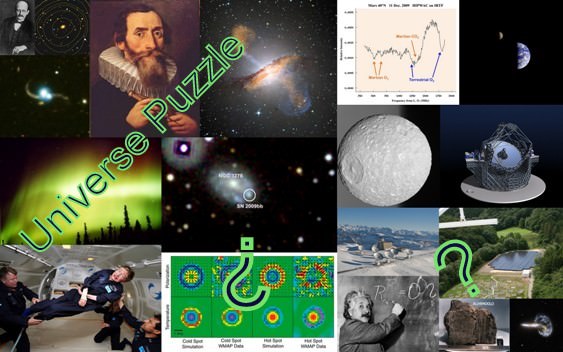
To start your working week, here’s a little something to help you sharpen your brain (OK, it’s already the end of the day for our viewers in New Zealand and Australia, so for you a little pick-me-up after a hard day’s work).
As with last week’s Universe Puzzle, something that cannot be answered by five minutes spent googling, a puzzle that requires you to cudgel your brains a bit, and do some lateral thinking. And a reminder: this is a puzzle on a “Universal” topic – astronomy and astronomers; space, satellites, missions, and astronauts; planets, moons, telescopes, and so on.
There are no prizes for the first correct answer – there may not even be just one correct answer! – posted as a comment (the judge’s decision – mine! – will be final!), but I do hope that you’ll have lots of fun.
What’s the next number in the sequence? 1655, 1671, 1672
Post your guesses in the comments section, and check back on Wednesday at this same post to find the answer. To make this puzzle fun for everyone, please don’t include links or extensive explanations with your answer, until after the answer has been given. Good luck!
PS There’s an open question on last week’s puzzle too (scroll down to the bottom of the comments).
UPDATE: Answer has been posted below.
Was this too easy perhaps? Maybe only five minutes’ spent googling was all that was needed to find the answer?
Christiaan Huygens discovered the first known moon of Saturn. The year was 1655 and the moon is Titan.
Giovanni Domenico Cassini made the next four discoveries: Iapetus (in 1671), Rhea (in 1672), …
… and Dione (in 1684), and Tethys (also in 1684).
What about Cassini’s discovery of the Cassini Division, in 1675?
Well, the discovery in 1655 was not made by Cassini, the rings of Saturn were discovered by Galileo (in 1610), and so on.
So, no, 1675 is not the next number in the sequence.
It’s amazing to reflect on how much more rapid astronomical discovery is, today, than back then; 45 years from the discovery of Saturn’s rings to Titan, another 20 to the discovery of the Cassini Division; 16 years between the discovery of Titan and Iapetus; … and 74 years from the rings to Dione and Tethys.
And today? Two examples: 45 years ago, x-ray astronomy was barely a toddler; and 74 years ago radio astronomy had just begun. Virtually all branches of astronomy outside the visual waveband went from scratch to today’s stunning results in less time than elapsed between the discovery of Saturn’s rings and its fourth brightest moon!
[/caption]
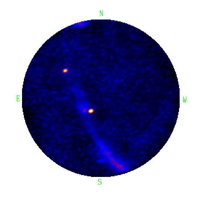
This image is a software-calibrated image with high signal-to-noise ratio at a frequency of 120 MHz, of the radio sky above Effelsberg, Germany, on November10, 2009. It has North at the top and East at the left, just as a person would have seen the entire sky when lying on their back on a flat field near Effelsberg late in the afternoon on November 10, if their eyes were sensitive to radio waves.
The two bright (yellow) spots are Cygnus A – a giant radio galaxy powered by a supermassive black hole – near the center of the image, and Cassiopeia A – a bright radio source created by a supernova explosion about 300 years ago – at the upper-left in the image. The plane of our Milky Way galaxy can also be seen passing by both Cassiopeia A and Cygnus A, and extending down to the bottom of the image. The North Polar Spur, a large cloud of radio emission within our own galaxy, can also be seen extending from the direction of the Galactic center in the South, toward the western horizon in this image. “We made this image with a single 60 second “exposure” at 120 MHz using our high-band LOFAR field in Effelsberg”, says James Anderson, project manager of the Effelsberg LOFAR station.
“The ability to make all-sky images in just seconds is a tremendous advancement compared to existing radio telescopes which often require weeks or months to scan the entire sky,” Anderson went on. This opens up exciting possibilities to detect and study rapid transient phenomena in the universe.
LOFAR, the LOw Frequency ARray, was designed and developed by ASTRON (Netherlands Institute for Radio Astronomy) with 36 stations centered on Exloo in the northeast of The Netherlands. It is now an international project with stations being built in Germany, France, the UK and Sweden connected to the central data processing facilities in Groningen (NL) and the ASTRON operations center in Dwingeloo (NL). The first international LOFAR station (IS-DE1) was completed on the area of the Effelsberg radio observatory next to the 100-m radio telescope of the Max-Planck-Institut für Radioastronomie (MPIfR).
Operating at relatively low radio frequencies from 10 to 240 MHz, LOFAR has essentially no moving parts to track objects in the sky; instead digital electronics are used to combine signals from many small antennas to electronically steer observations on the sky. In certain electronic modes, the signals from all of the individual antennas can be combined to make images of the entire radio sky visible above the horizon. IS-DE1: Some of the 96 low-band dipole antennas, Effelsberg LOFAR station (foreground); high-band array (background) (Credit: James Anderson, MPIfR)
LOFAR uses two different antenna designs, to observe in two different radio bands, the so-called low-band from 10 to 80 MHz, and the high-band from 110 to 240 MHz. All-sky images using the low-band antennas at Effelsberg were made in 2007.
Following the observation for the first high-band, all-sky image, scientists at MPIfR made a series of all-sky images covering a wide frequency range using both the low-band and high-band antennas at Effelsberg. Effelsberg sky through LOFAR eyes (Credit: James Anderson, MPIfR)
The movie of these all-sky images has been compiled and is shown above. The movie starts at a frequency of 35 MHz, and each subsequent frame is about 4 MHz higher in frequency, through 190 MHz. The resolution of the Effelsberg LOFAR telescope changes with frequency. At 35 MHz the resolution is about 10 degrees, at 110 MHz it is about 3.4 degrees, and at 190 MHz it is about 1.9 degrees. This change in resolution can be seen by the apparent size of the two bright sources Cygnus A and Cassiopeia A as the frequency changes.
Scientists at MPIfR and other institutions around Europe will use measurements such as these to study the large-sky structure of the interstellar matter of our Milky Way galaxy. The low frequencies observed by LOFAR are ideal for studying the low energy cosmic ray electrons in the Milky Way, which trace out magnetic field structures through synchrotron emission. Other large-scale features such as supernova remnants, star-formation regions, and even some other nearby galaxies will need similar measurements from individual LOFAR telescopes to provide accurate information on the large-scale emission in these objects. “We plan to search for radio transients using the all-sky imaging capabilities of the LOFAR telescopes”, says Michael Kramer, director at MPIfR, in Bonn. “The detection of rapidly variable sources using LOFAR could lead to exciting discoveries of new types of astronomical objects, similar to the discoveries of pulsars and gamma-ray bursts in the past decades.”
“The low-frequency sky is now truly open in Effelsberg and we have the capability at the observatory to observe in a wide frequency range from 10 MHz to 100 GHz”, says Anton Zensus, also director at MPIfR. “Thus we can cover four orders of magnitude in the electromagnetic spectrum.”
X-ray emission in the COSMOS field (XMM-Newton/ESA)
[/caption]
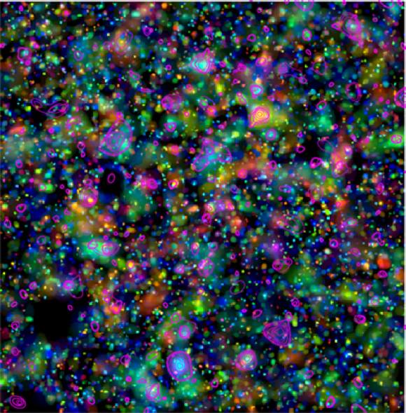
Galaxy density in the Cosmic Evolution Survey (COSMOS) field, with colors representing the redshift of the galaxies, ranging from redshift of 0.2 (blue) to 1 (red). Pink x-ray contours show the extended x-ray emission as observed by XMM-Newton.
Dark matter (actually cold, dark – non-baryonic – matter) can be detected only by its gravitational influence. In clusters and groups of galaxies, that influence shows up as weak gravitational lensing, which is difficult to nail down. One way to much more accurately estimate the degree of gravitational lensing – and so the distribution of dark matter – is to use the x-ray emission from the hot intra-cluster plasma to locate the center of mass.
And that’s just what a team of astronomers have recently done … and they have, for the first time, given us a handle on how dark matter has evolved over the last many billion years.
COSMOS is an astronomical survey designed to probe the formation and evolution of galaxies as a function of cosmic time (redshift) and large scale structure environment. The survey covers a 2 square degree equatorial field with imaging by most of the major space-based telescopes (including Hubble and XMM-Newton) and a number of ground-based telescopes.
Understanding the nature of dark matter is one of the key open questions in modern cosmology. In one of the approaches used to address this question astronomers use the relationship between mass and luminosity that has been found for clusters of galaxies which links their x-ray emissions, an indication of the mass of the ordinary (“baryonic”) matter alone (of course, baryonic matter includes electrons, which are leptons!), and their total masses (baryonic plus dark matter) as determined by gravitational lensing.
To date the relationship has only been established for nearby clusters. New work by an international collaboration, including the Max Planck Institute for Extraterrestrial Physics (MPE), the Laboratory of Astrophysics of Marseilles (LAM), and Lawrence Berkeley National Laboratory (Berkeley Lab), has made major progress in extending the relationship to more distant and smaller structures than was previously possible.
To establish the link between x-ray emission and underlying dark matter, the team used one of the largest samples of x-ray-selected groups and clusters of galaxies, produced by the ESA’s x-ray observatory, XMM-Newton.
Groups and clusters of galaxies can be effectively found using their extended x-ray emission on sub-arcminute scales. As a result of its large effective area, XMM-Newton is the only x-ray telescope that can detect the faint level of emission from distant groups and clusters of galaxies.
“The ability of XMM-Newton to provide large catalogues of galaxy groups in deep fields is astonishing,” said Alexis Finoguenov of the MPE and the University of Maryland, a co-author of the recent Astrophysical Journal (ApJ) paper which reported the team’s results.
Since x-rays are the best way to find and characterize clusters, most follow-up studies have until now been limited to relatively nearby groups and clusters of galaxies.
“Given the unprecedented catalogues provided by XMM-Newton, we have been able to extend measurements of mass to much smaller structures, which existed much earlier in the history of the Universe,” says Alexie Leauthaud of Berkeley Lab’s Physics Division, the first author of the ApJ study. COSMOS-XCL095951+014049 (Subaru/NAOJ, XMM-Newton/ESA)
Gravitational lensing occurs because mass curves the space around it, bending the path of light: the more mass (and the closer it is to the center of mass), the more space bends, and the more the image of a distant object is displaced and distorted. Thus measuring distortion, or ‘shear’, is key to measuring the mass of the lensing object.
In the case of weak gravitational lensing (as used in this study) the shear is too subtle to be seen directly, but faint additional distortions in a collection of distant galaxies can be calculated statistically, and the average shear due to the lensing of some massive object in front of them can be computed. However, in order to calculate the lens’ mass from average shear, one needs to know its center.
“The problem with high-redshift clusters is that it is difficult to determine exactly which galaxy lies at the centre of the cluster,” says Leauthaud. “That’s where x-rays help. The x-ray luminosity from a galaxy cluster can be used to find its centre very accurately.”
Knowing the centers of mass from the analysis of x-ray emission, Leauthaud and colleagues could then use weak lensing to estimate the total mass of the distant groups and clusters with greater accuracy than ever before.
The final step was to determine the x-ray luminosity of each galaxy cluster and plot it against the mass determined from the weak lensing, with the resulting mass-luminosity relation for the new collection of groups and clusters extending previous studies to lower masses and higher redshifts. Within calculable uncertainty, the relation follows the same straight slope from nearby galaxy clusters to distant ones; a simple consistent scaling factor relates the total mass (baryonic plus dark) of a group or cluster to its x-ray brightness, the latter measuring the baryonic mass alone.
“By confirming the mass-luminosity relation and extending it to high redshifts, we have taken a small step in the right direction toward using weak lensing as a powerful tool to measure the evolution of structure,” says Jean-Paul Kneib a co-author of the ApJ paper from LAM and France’s National Center for Scientific Research (CNRS).
The origin of galaxies can be traced back to slight differences in the density of the hot, early Universe; traces of these differences can still be seen as minute temperature differences in the cosmic microwave background (CMB) – hot and cold spots.
“The variations we observe in the ancient microwave sky represent the imprints that developed over time into the cosmic dark-matter scaffolding for the galaxies we see today,” says George Smoot, director of the Berkeley Center for Cosmological Physics (BCCP), a professor of physics at the University of California at Berkeley, and a member of Berkeley Lab’s Physics Division. Smoot shared the 2006 Nobel Prize in Physics for measuring anisotropies in the CMB and is one of the authors of the ApJ paper. “It is very exciting that we can actually measure with gravitational lensing how the dark matter has collapsed and evolved since the beginning.”
One goal in studying the evolution of structure is to understand dark matter itself, and how it interacts with the ordinary matter we can see. Another goal is to learn more about dark energy, the mysterious phenomenon that is pushing matter apart and causing the Universe to expand at an accelerating rate. Many questions remain unanswered: Is dark energy constant, or is it dynamic? Or is it merely an illusion caused by a limitation in Einstein’s General Theory of Relativity?
The tools provided by the extended mass-luminosity relationship will do much to answer these questions about the opposing roles of gravity and dark energy in shaping the Universe, now and in the future.
Sources: ESA, and a paper published in the 20 January, 2010 issue of the Astrophysical Journal (arXiv:0910.5219 is the preprint)
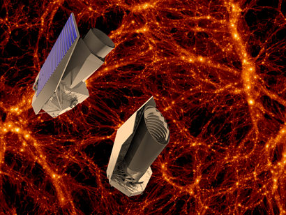
Thales Alenia Space and EADS Astrium concepts for Euclid (ESA)
Key questions relevant to fundamental physics and cosmology, namely the nature of the mysterious dark energy and dark matter (Euclid); the frequency of exoplanets around other stars, including Earth-analogs (PLATO); take the closest look at our Sun yet possible, approaching to just 62 solar radii (Solar Orbiter) … but only two! What would be your picks?
These three mission concepts have been chosen by the European Space Agency’s Science Programme Committee (SPC) as candidates for two medium-class missions to be launched no earlier than 2017. They now enter the definition phase, the next step required before the final decision is taken as to which missions are implemented.
These three missions are the finalists from 52 proposals that were either made or carried forward in 2007. They were whittled down to just six mission proposals in 2008 and sent for industrial assessment. Now that the reports from those studies are in, the missions have been pared down again. “It was a very difficult selection process. All the missions contained very strong science cases,” says Lennart Nordh, Swedish National Space Board and chair of the SPC.
And the tough decisions are not yet over. Only two missions out of three of them: Euclid, PLATO and Solar Orbiter, can be selected for the M-class launch slots. All three missions present challenges that will have to be resolved at the definition phase. A specific challenge, of which the SPC was conscious, is the ability of these missions to fit within the available budget. The final decision about which missions to implement will be taken after the definition activities are completed, which is foreseen to be in mid-2011.
[/caption] Euclid is an ESA mission to map the geometry of the dark Universe. The mission would investigate the distance-redshift relationship and the evolution of cosmic structures. It would achieve this by measuring shapes and redshifts of galaxies and clusters of galaxies out to redshifts ~2, or equivalently to a look-back time of 10 billion years. It would therefore cover the entire period over which dark energy played a significant role in accelerating the expansion.
By approaching as close as 62 solar radii, Solar Orbiter would view the solar atmosphere with high spatial resolution and combine this with measurements made in-situ. Over the extended mission periods Solar Orbiter would deliver images and data that would cover the polar regions and the side of the Sun not visible from Earth. Solar Orbiter would coordinate its scientific mission with NASA’s Solar Probe Plus within the joint HELEX program (Heliophysics Explorers) to maximize their combined science return. Thales Alenis Space concept, from assessment phase (ESA) PLATO (PLAnetary Transit and Oscillations of stars) would discover and characterize a large number of close-by exoplanetary systems, with a precision in the determination of mass and radius of 1%.
In addition, the SPC has decided to consider at its next meeting in June, whether to also select a European contribution to the SPICA mission.
SPICA would be an infrared space telescope led by the Japanese Space Agency JAXA. It would provide ‘missing-link’ infrared coverage in the region of the spectrum between that seen by the ESA-NASA Webb telescope and the ground-based ALMA telescope. SPICA would focus on the conditions for planet formation and distant young galaxies.
“These missions continue the European commitment to world-class space science,” says David Southwood, ESA Director of Science and Robotic Exploration, “They demonstrate that ESA’s Cosmic Vision programme is still clearly focused on addressing the most important space science.”
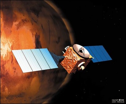
An illustration showing the ESA's Mars Express mission. Credit: ESA/Medialab)
Understanding the present-day Martian climate gives us insights into its past climate, which in turn provides a science-based context for answering questions about the possibility of life on ancient Mars.
Our understanding of Mars’ climate today is neatly packaged as climate models, which in turn provide powerful consistency checks – and sources of inspiration – for the climate models which describe anthropogenic global warming here on Earth.
But how can we work out what the climate on Mars is, today? A new, coordinated observation campaign to measure ozone in the Martian atmosphere gives us, the interested public, our own window into just how painstaking – yet exciting – the scientific grunt work can be.
[/caption]
The Martian atmosphere has played a key role in shaping the planet’s history and surface. Observations of the key atmospheric components are essential for the development of accurate models of the Martian climate. These in turn are needed to better understand if climate conditions in the past may have supported liquid water, and for optimizing the design of future surface-based assets at Mars.
Ozone is an important tracer of photochemical processes in the atmosphere of Mars. Its abundance, which can be derived from the molecule’s characteristic absorption spectroscopy features in spectra of the atmosphere, is intricately linked to that of other constituents and it is an important indicator of atmospheric chemistry. To test predictions by current models of photochemical processes and general atmospheric circulation patterns, observations of spatial and temporal ozone variations are required.
The Spectroscopy for Investigation of Characteristics of the Atmosphere of Mars (SPICAM) instrument on Mars Express has been measuring ozone abundances in the Martian atmosphere since 2003, gradually building up a global picture as the spacecraft orbits the planet.
These measurements can be complemented by ground-based observations taken at different times and probing different sites on Mars, thereby extending the spatial and temporal coverage of the SPICAM measurements. To quantitatively link the ground-based observations with those by Mars Express, coordinated campaigns are set up to obtain simultaneous measurements.
Infrared heterodyne spectroscopy, such as that provided by the Heterodyne Instrument for Planetary Wind and Composition (HIPWAC), provides the only direct access to ozone on Mars with ground-based telescopes; the very high spectral resolving power (greater than 1 million) allows Martian ozone spectral features to be resolved when they are Doppler shifted away from ozone lines of terrestrial origin.
A coordinated campaign to measure ozone in the atmosphere of Mars, using SPICAM and HIPWAC, has been ongoing since 2006. The most recent element of this campaign was a series of ground-based observations using HIPWAC on the NASA Infrared Telescope Facility (IRTF) on Mauna Kea in Hawai’i. These were obtained between 8 and 11 December 2009 by a team of astronomers led by Kelly Fast from the Planetary Systems Laboratory, at NASA’s Goddard Space Flight Center (GSFC), in the USA. Credit: Kelly Fast About the image: HIPWAC spectrum of Mars’ atmosphere over a location on Martian latitude 40°N; acquired on 11 December 2009 during an observation campaign with the IRTF 3 m telescope in Hawai’i. This unprocessed spectrum displays features of ozone and carbon dioxide from Mars, as well as ozone in the Earth’s atmosphere through which the observation was made. Processing techniques will model and remove the terrestrial contribution from the spectrum and determine the amount of ozone at this northern position on Mars.
The observations had been coordinated in advance with the Mars Express science operations team, to ensure overlap with ozone measurements made in this same period with SPICAM.
The main goal of the December 2009 campaign was to confirm that observations made with SPICAM (which measures the broad ozone absorption spectra feature centered at around 250 nm) and HIPWAC (which detects and measures ozone absorption features at 9.7 μm) retrieve the same total ozone abundances, despite being performed at two different parts of the electromagnetic spectrum and having different sensitivities to the ozone profile. A similar campaign in 2008, had largely validated the consistency of the ozone measurement results obtained with SPICAM and the HIPWAC instrument.
The weather conditions and the seeing were very good at the IRTF site during the December 2009 campaign, which allowed for good quality spectra to be obtained with the HIPWAC instrument.
Kelly and her colleagues gathered ozone measurements for a number of locations on Mars, both in the planet’s northern and southern hemisphere. During this four-day campaign the SPICAM observations were limited to the northern hemisphere. Several HIPWAC measurements were simultaneous with observations by SPICAM allowing a direct comparison. Other HIPWAC measurements were made close in time to SPICAM orbital passes that occurred outside of the ground-based telescope observations and will also be used for comparison.
The team also performed measurements of the ozone abundance over the Syrtis Major region, which will help to constrain photochemical models in this region.
Analysis of the data from this recent campaign is ongoing, with another follow-up campaign of coordinated HIPWAC and SPICAM observations already scheduled for March this year.
Putting the compatibility of the data from these two instruments on a firm base will support combining the ground-based infrared measurements with the SPICAM ultraviolet measurements in testing the photochemical models of the Martian atmosphere. The extended coverage obtained by combining these datasets helps to more accurately test predictions by atmospheric models.
It will also quantitatively link the SPICAM observations to longer-term measurements made with the HIPWAC instrument and its predecessor IRHS (the Infrared Heterodyne Spectrometer) that go back to 1988. This will support the study of the long-term behavior of ozone and associated chemistry in the atmosphere of Mars on a timescale longer than the current missions to Mars.
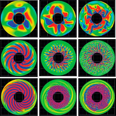
Zonal swishing in the Earth's outer core (Credit: Akira Kageyama, Kobe University)
[/caption]
Why does the Earth’s magnetic field ‘flip’ every million years or so? Whatever the reason, or reasons, the way the liquid iron of the Earth’s outer core flows – its currents, its structure, its long-term cycles – is important, either as cause, effect, or a bit of both.
The main component of the Earth’s field – which defines the magnetic poles – is a dipole generated by the convection of molten nickel-iron in the outer core (the inner core is solid, so its role is secondary; remember that the Earth’s core is well above the Curie temperature, so the iron is not ferromagnetic).
But what about the fine structure? Does the outer core have the equivalent of the Earth’s atmosphere’s jet streams, for example? Recent research by a team of geophysicists in Japan sheds some light on these questions, and so hints at what causes magnetic pole flips.
About the image: This image shows how an imaginary particle suspended in the liquid iron outer core of the Earth tends to flow in zones even when conditions in the geodynamo are varied. The colors represent the vorticity or “amount of rotation” that this particle experiences, where red signifies positive (east-west) flow and blue signifies negative (west-east) flow. Left to right shows how the flow responds to increasing Rayleigh numbers, which is associated with flow driven by buoyancy. Top to bottom shows how flow responds to increasing angular velocities of the whole geodynamo system.
The jet stream winds that circle the globe and those in the atmospheres of the gas giants (Jupiter, Saturn, etc) are examples of zonal flows. “A common feature of these zonal flows is that they are spontaneously generated in turbulent systems. Because the Earth’s outer core is believed to be in a turbulent state, it is possible that there is zonal flow in the liquid iron of the outer core,” Akira Kageyama at Kobe University and colleagues say, in their recent Nature paper. The team found a secondary flow pattern when they modeled the geodynamo – which generates the Earth’s magnetic field – to build a more detailed picture of convection in the Earth’s outer core, a secondary flow pattern consisting of inner sheet-like radial plumes, surrounded by westward cylindrical zonal flow.
This work was carried out using the Earth Simulator supercomputer, based in Japan, which offered sufficient spatial resolution to determine these secondary effects. Kageyama and his team also confirmed, using a numerical model, that this dual-convection structure can co-exist with the dominant convection that generates the north and south poles; this is a critical consistency check on their models, “We numerically confirm that the dual-convection structure with such a zonal flow is stable under a strong, self-generated dipole magnetic field,” they write.
This kind of zonal flow in the outer core has not been seen in geodynamo models before, due largely to lack of sufficient resolution in earlier models. What role these zonal flows play in the reversal of the Earth’s magnetic field is one area of research that Kageyama and his team’s results that will now be able to be pursued.
[/caption]
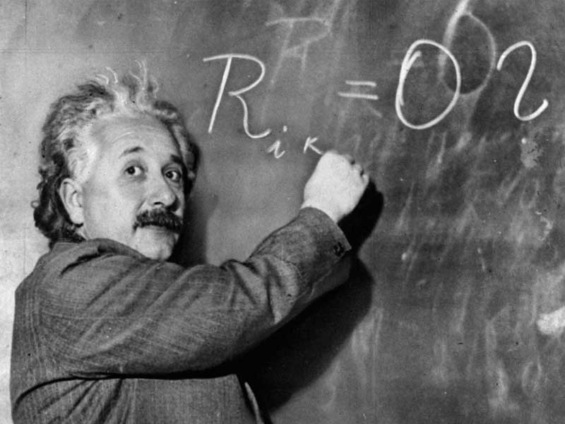
This time it was the gravitational redshift part of General Relativity; and the stringency? An astonishing better-than-one-part-in-100-million!
How did Steven Chu (US Secretary of Energy, though this work was done while he was at the University of California Berkeley), Holger Müler (Berkeley), and Achim Peters (Humboldt University in Berlin) beat the previous best gravitational redshift test (in 1976, using two atomic clocks – one on the surface of the Earth and the other sent up to an altitude of 10,000 km in a rocket) by a staggering 10,000 times?
By exploited wave-particle duality and superposition within an atom interferometer!
Cesium atom interferometer test of gravitational redshift (Courtesy Nature) About this figure: Schematic of how the atom interferometer operates. The trajectories of the two atoms are plotted as functions of time. The atoms are accelerating due to gravity and the oscillatory lines depict the phase accumulation of the matter waves. Arrows indicate the times of the three laser pulses. (Courtesy: Nature).
Gravitational redshift is an inevitable consequence of the equivalence principle that underlies general relativity. The equivalence principle states that the local effects of gravity are the same as those of being in an accelerated frame of reference. So the downward force felt by someone in a lift could be equally due to an upward acceleration of the lift or to gravity. Pulses of light sent upwards from a clock on the lift floor will be redshifted when the lift is accelerating upwards, meaning that this clock will appear to tick more slowly when its flashes are compared at the ceiling of the lift to another clock. Because there is no way to tell gravity and acceleration apart, the same will hold true in a gravitational field; in other words the greater the gravitational pull experienced by a clock, or the closer it is to a massive body, the more slowly it will tick.
Confirmation of this effect supports the idea that gravity is geometry – a manifestation of spacetime curvature – because the flow of time is no longer constant throughout the universe but varies according to the distribution of massive bodies. Exploring the idea of spacetime curvature is important when distinguishing between different theories of quantum gravity because there are some versions of string theory in which matter can respond to something other than the geometry of spacetime.
Gravitational redshift, however, as a manifestation of local position invariance (the idea that the outcome of any non-gravitational experiment is independent of where and when in the universe it is carried out) is the least well confirmed of the three types of experiment that support the equivalence principle. The other two – the universality of freefall and local Lorentz invariance – have been verified with precisions of 10-13 or better, whereas gravitational redshift had previously been confirmed only to a precision of 7×10⁻⁵.
In 1997 Peters used laser trapping techniques developed by Chu to capture cesium atoms and cool them to a few millionths of a degree K (in order to reduce their velocity as much as possible), and then used a vertical laser beam to impart an upward kick to the atoms in order to measure gravitational freefall.
Now, Chu and Müller have re-interpreted the results of that experiment to give a measurement of the gravitational redshift.
In the experiment each of the atoms was exposed to three laser pulses. The first pulse placed the atom into a superposition of two equally probable states – either leaving it alone to decelerate and then fall back down to Earth under gravity’s pull, or giving it an extra kick so that it reached a greater height before descending. A second pulse was then applied at just the right moment so as to push the atom in the second state back faster toward Earth, causing the two superposition states to meet on the way down. At this point the third pulse measured the interference between these two states brought about by the atom’s existence as a wave, the idea being that any difference in gravitational redshift as experienced by the two states existing at difference heights above the Earth’s surface would be manifest as a change in the relative phase of the two states.
The virtue of this approach is the extremely high frequency of a cesium atom’s de Broglie wave – some 3×1025Hz. Although during the 0.3 s of freefall the matter waves on the higher trajectory experienced an elapsed time of just 2×10-20s more than the waves on the lower trajectory did, the enormous frequency of their oscillation, combined with the ability to measure amplitude differences of just one part in 1000, meant that the researchers were able to confirm gravitational redshift to a precision of 7×10⁻⁹.
As Müller puts it, “If the time of freefall was extended to the age of the universe – 14 billion years – the time difference between the upper and lower routes would be a mere one thousandth of a second, and the accuracy of the measurement would be 60 ps, the time it takes for light to travel about a centimetre.”
Müller hopes to further improve the precision of the redshift measurements by increasing the distance between the two superposition states of the cesium atoms. The distance achieved in the current research was a mere 0.1 mm, but, he says, by increasing this to 1 m it should be possible to detect gravitational waves, predicted by general relativity but not yet directly observed.
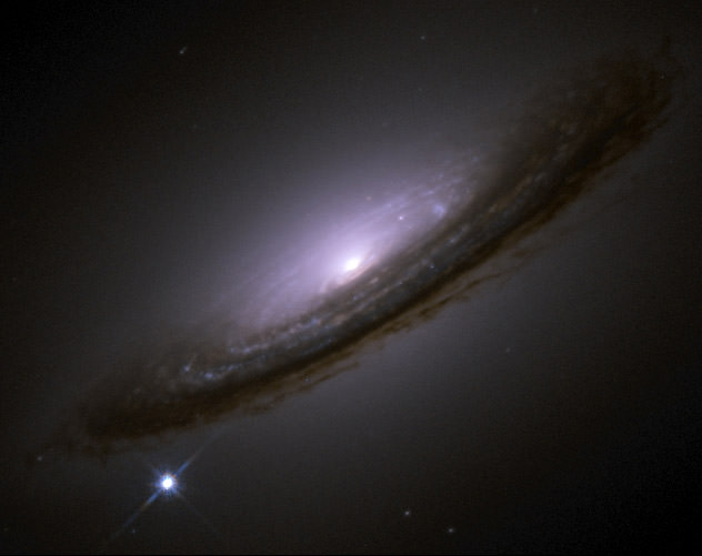
[/caption]
What is a supernova? Well, “nova” means “new star”, and “super” means “really big”, like supermarket, so a supernova is a really bright new star. That’s where the word comes from, but today it has a rather more precise meaning, namely a once-off variable star which has a peak brightness similar to, or greater than, that of a typical galaxy.
Supernovae aren’t new stars in the sense that they were not stars before they became supernovae; the progenitor – what the star was before it went supernova – of a supernova is just a star (or a pair of stars), albeit an unusual one.
From what we see – the rise of the intensity of light (and electromagnetic radiation in general) to a peak, its decline; the lines which show up in the spectra (and the ones which don’t), etc – we can classify supernovae into several different types. There are two main types, called Type I and Type II. The difference between them is that Type I supernovae have no lines of hydrogen in their spectra, while Type II ones do.
Centuries of work by astronomers and physicists have given us just two kinds of progenitors: white dwarfs and massive (>8 sols) stars; and just two key physical mechanisms: nuclear detonation and core collapse.
Core collapse supernovae happen when a massive star tries to fuse iron in its core … bad move, because fusing iron requires energy (rather than liberates it), and the core suddenly collapses due to its gravity. A lot of interesting physics happens when such a core collapses, but it either results in a neutron star or a black hole, and a vast amount of energy is produced (most of it in the form of neutrinos!). These supernovae can be of any type, except a sub-type of Type I (called Ia). They also produce the long gamma-ray bursts (GRB).
Detonation is when a white dwarf star undergoes almost simultaneous fusion of carbon or oxygen throughout its entire body (it can do this because a white dwarf has the same temperature throughout, unlike an ordinary star, because its electrons are degenerate). There are at least two ways such a detonation can be triggered: steady accumulation of hydrogen transferred from a close binary companion, or a collision or merger with a neutron star or another white dwarf. These supernovae are all Type Ia.
One other kind of supernova: when two neutron stars merge, or a ~solar mass black hole and a neutron star merge – as a result of loss of orbital energy due to gravitational wave radiation – an intense burst of gamma-rays results, along with a fireball and an afterglow (as the fireball cools). We see such an event as a short GRB, but if we were unlikely enough to be close to such a stellar death, we’d certainly see it as a spectacular supernova!
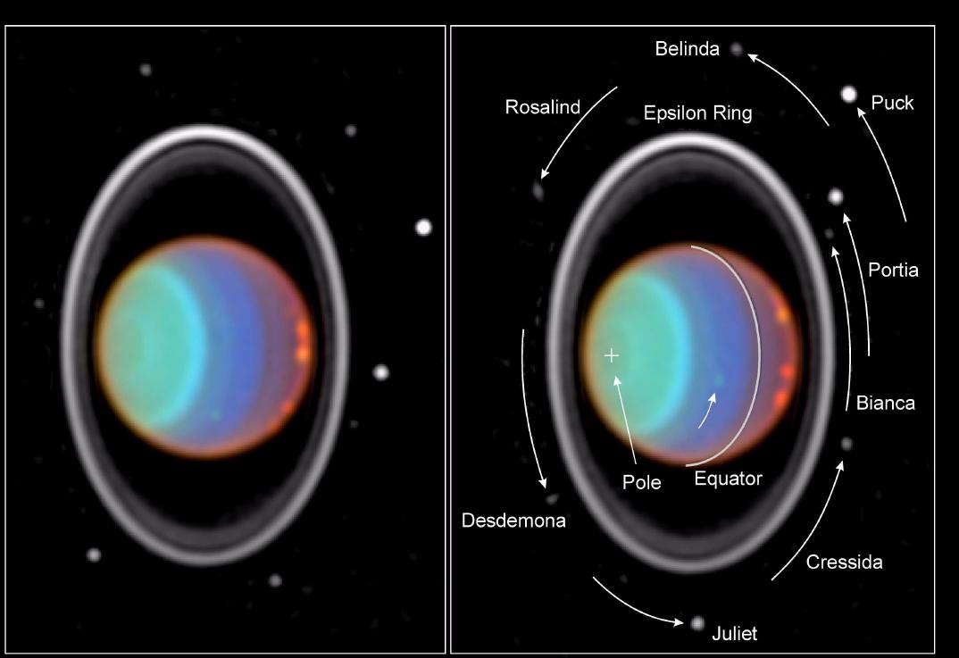
Uranus with its moons and rings. Image credit: Hubble
[/caption]
The Roche limit is named after French astronomy Edouard Roche, who published the first calculation of the theoretical limit, in 1848. The Roche limit is a distance, the minimum distance that a smaller object (e.g. a moon) can exist, as a body held together by its self-gravity, as it orbits a more massive body (e.g. its parent planet); closer in, and the smaller body is ripped to pieces by the tidal forces on it.
Remember how tidal forces come about? Gravity is an inverse-square-law force – twice as far away and the gravitational force is four times as weak, for example – so the gravitational force due to a planet, say, is greater on one of its moon’s near-side (the side facing the planet) than its far-side.
The fine details of whether an object can, in fact, hold up against the tidal force of its massive neighbor depend on more than just the self-gravity of the smaller body. For example, an ordinary star is much more easily ripped to piece by tidal forces – due to a supermassive black hole, say – than a ball of pure diamond (which is held together by the strength of the carbon-carbon bonds, in addition to its self-gravity).
The best known application of Roche’s theoretical work is on the formation of planetary rings: an asteroid or comet which strays within the Roche limit of a planet will disintegrate, and after a few orbits the debris will form a nice ring around the planet (of course, this is not the only way a planetary ring can form; small moons can create rings by being bombarded by micrometeorites, or by outgassing).
Roche also left us with two other terms widely used in astronomy and astrophysics, Roche lobe and Roche sphere; no surprise to learn that they too refer to gravity in systems of two bodies!
[/caption]
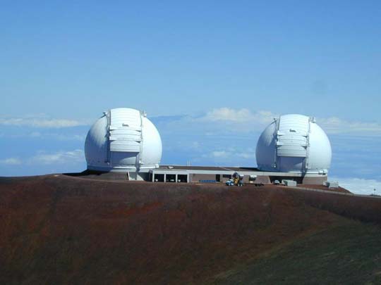
There are two Keck telescopes – Keck I and Keck II; together they make up the W.M. Keck Observatory, though strictly speaking the observatory is a great deal more than just the telescopes (there’s all the instrumentation, especially the interferometer, the staff, support facilities, etc, etc, etc.).
William Myron Keck (1880-1964) established a philanthropic foundation in 1954, to support scientific discoveries and new technologies. One project funded was the first Keck telescope, which was quite revolutionary at the time. Not only was it the largest optical telescope (and it still is) – it’s 10 meters in diameter – but is made up of 36 hexagonal segments, the manufacture of which required several breakthroughs … and all 36 are kept in line by a system of sensors and actuators which adjusts their position twice a second. Keck I saw first light in 1993. Like nearly all modern, large optical telescopes, the Keck telescopes are alt-azimuth. Fun fact: to keep the telescope at an optimal working temperature – no cool-down period during the evening – giant aircons work flat out during the day.
The Keck telescopes are on the summit of Hawaii’s Mauna Kea, where the air is nearly always clear, dry, and not turbulent (the seeing is, routinely, below 1″); an ideal site for not only optical astronomy, but also infrared.
The second Keck telescope – Keck II – saw first light in 1996, but its real day of glory came in 1999, when one of the first adaptive optics (AO) systems was installed on it (the first installed on a large telescope).
2004 saw another first for the Keck telescope – a laser guide star AO system, which gives the Keck telescopes a resolution at least as good as the Hubble Space Telescope’s (in the infrared)!
And in 2005 the two Keck telescopes operated together, as an interferometer; yet another first.

; high-band array (background) (Credit: James Anderson, MPIfR)")
")
")
")

")