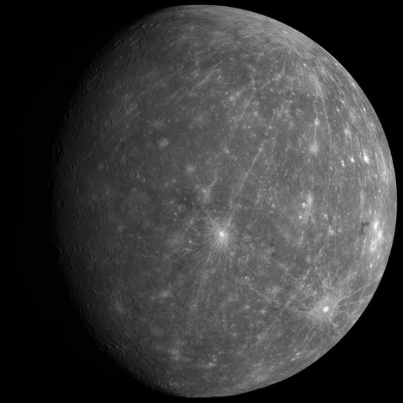
Mosaic of Mercury. Credit: NASA / JHUAPL / CIW / mosaic by Jason Perry
Mercury is one of the most unusual planets in our Solar System, at least by the standards of us privileged Earthlings. Despite being the closest planet to our Sun, it is not the hottest (that honor goes to Venus). And because of its virtually non-existence atmosphere and slow rotation, temperatures on its surface range from being extremely hot to extremely cold.
Equally unusual is the diurnal cycle on Mercury – i.e. the cycle of day and night. A single year lasts only 88 days on Mercury, but thanks again to its slow rotation, a day lasts twice as long! That means that if you could stand on the surface of Mercury, it would take a staggering 176 Earth days for the Sun to rise, set and rise again to the same place in the sky just once!
Distance and Orbital Period:
Mercury is the closest planet to our Sun, but it also has the most eccentric orbit (0.2056) of any of the Solar Planets. This means that while its average distance (semi-major axis) from the Sun is 57,909,050 km (35,983,015 mi) or 0.387 AUs, this ranges considerably – from 46,001,200 km (2,8583,820 mi) at perihelion (closet) to 69,816,900 km (43,382,210 mi) at aphelion (farthest).
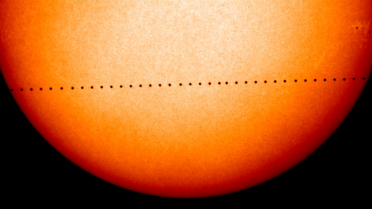
A timelapse of Mercury transiting across the face of the Sun. Credit: NASA
Because of this proximity, Mercury has a rapid orbital period, which varies depending on where it is in its orbit. Naturally, it moves fastest when it is at its closest to the Sun, and slowest when it is farthest. On average, its orbital velocity is 47.362 km/s (29.43 mi/s), which means it takes only 88 days to complete a single orbit of the Sun.
Astronomers used to suspect that Mercury was tidally locked to the Sun, meaning that it always showed the same face to the Sun – similar to how the Moon is tidally locked to the Earth. But radar-Doppler measurements obtained in 1965 demonstrated that Mercury is actually rotating very slowly compared to the Sun.
Sidereal vs. Solar Day:
Based on data obtained by these radar measurements, Mercury is now known to be in 3:2 orbital resonance with the Sun. This means that the planet completes three rotations on its axis for every two orbits it makes around the Sun. At it’s current rotational velocity – 3.026 m/s, or 10.892 km/h (6.77 mph) – it takes Mercury 58.646 days to complete a single rotation on its axis.
While this might lead some to conclude that a single day on Mercury is about 58 Earth days – thus making the length of a day and year correspond to the same 3:2 ratio – this would be inaccurate. Due to its rapid orbital velocity and slow sidereal rotation, a Solar Day on Mercury (the time it takes for the Sun to return to the same place in the sky) is actually 176 days.
In that respect, the ratio of days to years on Mercury is actually 1:2. The only places that are exempt to this day and night cycle are the polar regions. The cratered northern polar region, for example, exists in a state of perpetual shadow. Temperatures in these craters are also cool enough that significant concentrations of water ice can exist in stable form.
For over 20 years, scientists believed that radar-bright images from Mercury’s northern polar regions might indicate the presence of water ice there. In November of 2012, NASA’s MESSENGER probe examined the northern polar region using its neutron spectrometer and laser altimeter and confirmed the presence of both water ice and organic molecules.
View of Mercury’s north pole. based on MESSENGER probe data, showing polar deposits of water ice. Credit: NASA/JHUAPL/Carnegie Institute of Science/NAIC/Arecibo Observatory
Yes, as if Mercury weren’t strange enough, it turns out that a single day on Mercury lasts as long as two years! Just another oddity for a planet that likes to keep things really hot, really cold, and is really eccentric.
ASA's Cassini spacecraft looks toward the night side of Saturn's largest moon and sees sunlight scattering through the periphery of Titan's atmosphere and forming a ring of color.
Credit: NASA/JPL-Caltech/Space Science Institute
Last week – from Monday, February 27th to Wednesday, March 1st – NASA hosted the “Planetary Science Vision 2050 Workshop” at their headquarters in Washington, DC. In the course of the many presentations, speeches and panel discussions, NASA’s shared its many plans for the future of space exploration with the international community.
Among the more ambitious of these was a proposal to explore Titan using an aerial explorer and a lander. Building upon the success of the ESA’s Cassini-Huygen mission, this plan would involve a balloon that would explore Titan’s surface from low altitude, along with a Mars Pathfinder-style mission that would explore the surface.
Ultimately, the goal a mission to Titan would be to explore the rich organic chemical environment the moon has, which presents a unique opportunity for planetary researchers. For some time, scientists have understood that Titan’s surface and atmosphere have an abundance of organic compounds and all the prebiotic chemistry necessary for life to function.
Artist depiction of Huygens landing on Titan. Credit: ESA
“Titan’s of particular interest because the abundant and complex organic chemistry can teach us about chemical interactions that could have occurred here on Earth (and elsewhere?) leading to the development of life. Furthermore, not only does Titan have an interior liquid-water ocean, but there will also have been opportunities for organic material to have mixed with liquid water at Titan’s surface, for example impact craters and possibly cryovolcanic eruptions. The combination of organic material with liquid water, of course, increases astrobiological potential.”
For this reason, the exploration of Titan has been a scientific goal for decades. The only question is how best to go about exploring Titan’s unique environment. During previous Decadal Surveys – such as the Campaign Strategy Working Group (CSWG) on Prebiotic Chemistry in the Outer Solar System, of which Lorenz was a contributor – has suggested that a mobile aerial vehicle (such as an airship or a balloon) would well-suited to the task.
However, such vehicles would be unable to study Titan’s methane lakes, which are one of the most exciting draws of the moon as far as research into prebiotic chemistry goes. What’s more, an aerial vehicle would not be able to conduct in-situ chemical analysis of the surface, much like what the Mars Exploration Rovers (Spirit, Opportunity and Curiosity) have been doing on Mars – and with immense results!
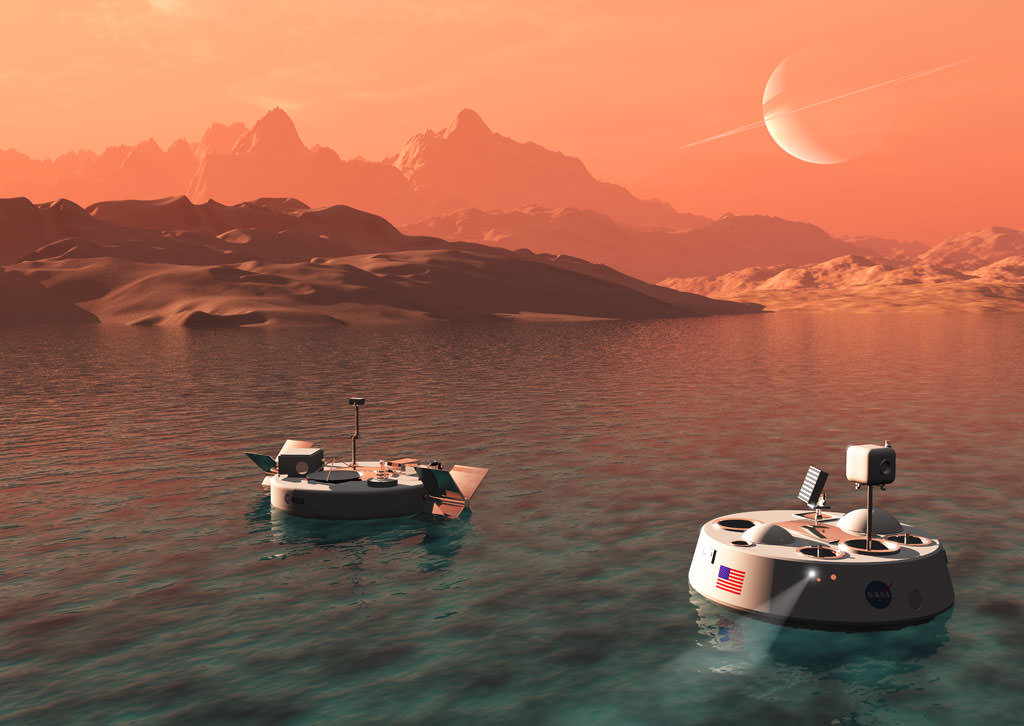
The ESA’s TALISE (Titan Lake In-situ Sampling Propelled Explorer) on the left, and NASA’s Titan Mare Explorer (TiME) on the right. Credit: bisbos.com
At the same time, Lorenz and his colleagues examined concepts for the exploration of Titan’s hydrocarbon seas – like the proposed Titan Mare Explorer (TiME) capsule. As one of several finalists of NASA’s 2010 Discovery competition, this concept called for the deployment of nautical robot to Titan in the coming decades, where it would study its methane lakes to learn more about the methane cycle and search for signs of organic life.
While such a proposal would be cost-effective and presents some very exciting opportunities for research, it also has some limitations. For instance, during the 2020s-2030s, Titan’s northern hemisphere will be experiencing its winter season; at which point the thickness of its atmosphere will make direct-to-Earth communications and Earth views impossible. On top of that, a nautical vehicle would preclude the exploration of Titan’s land surfaces.
These offer some of the most likely prospects for studying Titan’s advanced chemical evolution, including Titan’s dune sands. As a windswept region, this area likely has material deposited from all over Titan and may also contain aqueously altered materials. Much as the Mars Pathfinder landing site was selected so it could collect samples from a wide area, such as location would be an ideal site for a lander.
As such, Lorenz and his colleagues advocated the type of mission that was articulated in the 2007 Flagship Study, which called for a Montgolfière balloon for regional exploration and a Pathfinder-like lander. This would provide the opportunity to conduct surface imaging at resolutions that are impossible from orbit (due to the thick atmosphere) as well as investigating the surface chemistry and interior structure of the moon.
Artist’s conception of a possible structure for underground liquid reservoirs on Saturn moon’s Titan. Credit: ESA/ATG medialab
So while the balloon would gather high-resolution geographical data of the moon, the lander could conduct seismological surveys that would characterize the thickness of the ice above Titan’s internal water ocean. However, a lander mission would be limited in terms of range, and the surface of Titan presents problems for mobility. This would make multiple landers, or a relocatable lander, the most desired option.
“Potential targets include areas where we can measure solid surface materials, the composition of which is still not well known, Titan’s dune sands, for example,” said Turtle. “Detailed in situ analysis is required to determine their composition. The lakes and seas are also intriguing; however, in the nearer term (missions arriving in the 2030s) most of those will be in winter darkness. So, exploring them would likely have to wait until the 2040s.”
This mission concept would also take advantage of several technological advances that have been made in recent years. As Lorenz explained in the course of the presentation:
“Heavier-than-air mobility at Titan is in fact highly efficient, moreover, improvements in autonomous aircraft in the two decades since the CSWG make such exploration a realistic prospect. Multiple in-situ landers delivered by an aerial vehicle like an airplane or a lander with aerial mobility to access multiple sites, would provide the most desirable scientific capability, highly relevant to the themes of origins, workings, and life.”
Updated maps of Titan, based on the Cassini imaging science subsystem. Credit: NASA/JPL/Space Science Institute
However, addressing some additional challenges not raised at the 2050 Vision Workshop, they will be presenting a slight twist on their idea. Instead of a balloon and multiple landers, they will present a mission concept involving a “Dragonfly” qaudcopter. This four-rotor vehicle would be able to take advantage of Titan’s thick atmosphere and low gravity to obtain samples and determine the surface composition in multiple geological settings.
This concept also incorporates a lot of recent advances in technology, which include modern control electronics and advances in commerical unmanned aerial vehicle (UAV) designs. On top of that, a quadcopter would do away with chemically-powered retrorockets and could power-up between flights, giving it a potentially much longer lifespan.
These and other concepts for exploring Saturn’s moon Titan are sure to gain traction in the coming years. Given the many mysteries locked away on this world – with includes abundant water ice, prebiotic chemistry, a methane cycle, and a subsurface ocean that is likely to be a prebiotic environment – it is certainly a popular target for scientific research.
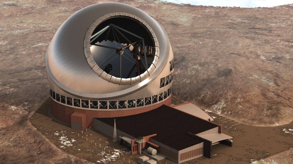
An artist's illustration of the Thirty Meter Telescope at its preferred location at Mauna Kea, Hawaii. Image Courtesy TMT International Observatory
As Carl Sagan said, “Understanding is Ecstasy.” But in order to understand the Universe, we need better and better ways to observe it. And that means one thing: big, huge, enormous telescopes.
In this series, we’ll look at six Super Telescopes being built:
The Thirty Meter Telescope (TMT) is being built by an international group of countries and institutions, like a lot of Super Telescopes are. In fact, they’re proud of pointing out that the international consortium behind the TMT represents almost half of the world’s population; China, India, the USA, Japan, and Canada. The project needs that many partners to absorb the cost; an estimated $1.5 billion.
The heart of any of the world’s Super Telescopes is the primary mirror, and the TMT is no different. The primary mirror for the TMT is, obviously, 30 meters in diameter. It’s a segmented design consisting of 492 smaller mirrors, each one a 1.4 meter hexagon.
The light collecting capability of the TMT will be 10 times that of the Keck Telescope, and more than 144 times that of the Hubble Space Telescope.
But the TMT is more than just an enormous ‘light bucket.’ It also excels with other capabilities that define a super telescope’s effectiveness. One of those is what’s called diffraction-limited spatial resolution (DLSR).
An illustration of the segmented primary mirror of the Thirty Meter Telescope. Image Courtesy TMT International Observatory
When a telescope is pointed at distant objects that appear close together, the light from both can scatter enough to make the two objects appear as one. Diffraction-limited spatial resolution means that when a ‘scope is observing a star or other object, none of the light from that object is scattered by defects in the telescope. The TMT will more easily distinguish objects that are close to each other. When it comes to DLSR, the TMT will exceed the Keck by a factor of 3, and will exceed the Hubble by a factor of 10 at some wavelengths.
Crucial to the function of large, segmented mirrors like the TMT is active optics. By controlling the shape and position of each segment, active optics allows the primary mirror to compensate for changes in wind, temperature, or mechanical stress on the telescope. Without active optics, and its sister technology adaptive optics, which compensates for atmospheric disturbance, any telescope larger than about 8 meters would not function properly.
The TMT will operate in the near-ultraviolet, visible, and near-infrared wavelengths. It will be smaller than the European Extremely Large Telescope (E-ELT), which will have a 39 meter primary mirror. The E-ELT will operate in the optical and infrared wavelengths.
The world’s Super Telescopes are behemoths. Not just in the size of their mirrors, but in their mass. The TMT’s moving mass will be about 1,420 tonnes. Moving the TMT quickly is part of the design of the TMT, because it must respond quickly when something like a supernova is spotted. The detailed science case calls for the TMT to acquire a new target within 5 to 10 minutes.
This requires a complex computer system to coordinate the science instruments, the mirrors, the active optics, and the adaptive optics. This was one of the initial challenges of the TMT project. It will allow the TMT to respond to transient phenomena like supernovae when spotted by other telescopes like the Large Synoptic Survey Telescope.
The Science
The TMT will investigate most of the important questions in astronomy and cosmology today. Here’s an overview of major topics that the TMT will address:
The Nature of Dark Matter
The Physics of Extreme Objects like Neutron Stars
Early galaxies and Cosmic Reionization
Galaxy Formation
Super-Massive Black Holes
Exploration of the Milky Way and Nearby Galaxies
The Birth and Early Lives of Stars and Planets
Time Domain Science: Supernovae and Gamma Ray Bursts
Exo-planets
Our Solar System
This is a comprehensive list of topics, to be sure. It leaves very little out, and is a testament to the power and effectiveness of the TMT.
The raw power of the TMT is not in question. Once in operation it will advance our understanding of the Universe on multiple fronts. But the actual location of the TMT could still be in question.
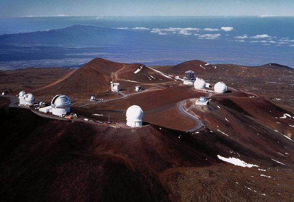
The top of Mauna Kea is a prime site for telescopes, as shown in this image. Image Courtesy Mauna Kea Observatories
The dispute between some of the Hawaiian people and the TMT has been well-documented elsewhere, but the basic complaint about the TMT is that the top of Mauna Kea is sacred land, and they would like the TMT to be built elsewhere.
The organizations behind the TMT would still like it to be built at Mauna Kea, and a legal process is unfolding around the dispute. During that process, they identified several possible alternate sites for the telescope, including La Palma in the Canary Islands. Universe Today contacted TMT Observatory Scientist Christophe Dumas, PhD., about the possible relocation of the TMT to another site.
Dr. Dumas told us that “Mauna Kea remains the preferred location for the TMT because of its superb observing conditions, and because of the synergy with other TMT partner facilities already present on the mountain. Its very high elevation of almost 14,000 feet makes it the premier astronomical site in the northern hemisphere. The sky above Mauna Kea is very stable, which allows very sharp images to be obtained. It has also excellent transparency, low light pollution and stable cold temperatures that improves sensitivity for observations in the infrared.”
The preferred secondary site at La Palma is home to over 10 other telescopes, but would relocation to the Canary Islands affect the science done by the TMT? Dr. Dumas says that the Canary Islands site is excellent as well, with similar atmospheric characteristics to Mauna Kea, including stability, transparency, darkness, and fraction of clear-nights.
The Gran Telescopio Canarias (Great Canary Telescope) is the largest ‘scope currently at La Palma. At 10m diameter, it would be dwarfed by the TMT. Image: By Pachango – Own work, CC BY-SA 3.0, https://commons.wikimedia.org/w/index.php?curid=6880933
As Dr. Dumas explains, “La Palma is at a lower elevation site and on average warmer than Mauna Kea. These two factors will reduce TMT sensitivity at some wavelengths in the infrared region of the spectrum.”
Dr. Dumas told Universe Today that this reduced sensitivity in the infrared can be overcome somewhat by scheduling different observing tasks. “This specific issue can be partly mitigated by implementing an adaptive scheduling of TMT observations, to match the execution of the most demanding infrared programs with the best atmospheric conditions above La Palma.”
Court Proceedings End
On March 3rd, 44 days of court hearings into the TMT wrapped up. In that time, 71 people testified for and against the TMT being constructed on Mauna Kea. Those against the telescope say that the site is sacred land and shouldn’t have any more telescope construction on it. Those for the TMT spoke in favor of the science that the TMT will deliver to everyone, and the education opportunities it will provide to Hawaiians.
Though construction has been delayed, and people have gone to court to have the project stopped, it seems like the TMT will definitely be built—somewhere. The funding is in place, the design is finalized, and manufacturing of the components is underway. The delays mean that the TMT’s first light is still uncertain, but once we get there, the TMT will be another game-changer, just like the world’s other Super Telescopes.
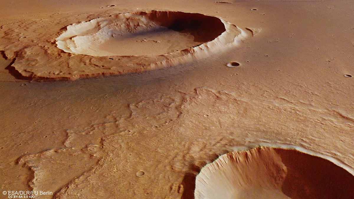
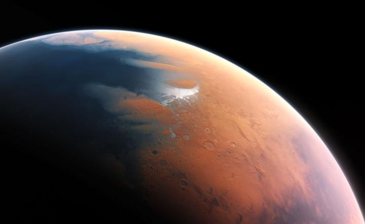
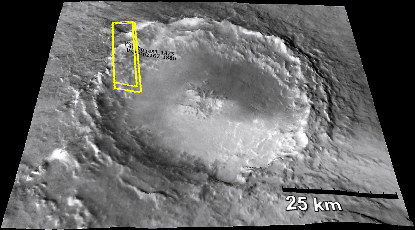
Perspective view looking from an unnamed crater (bottom right) towards the Worcester Crater. The region sits at the mouth of Kasei Valles, where fierce floodwaters emptied into Chryse Planitia. Credit: ESA/DLR/FU Berlin
The Mars Express probe was the European Space Agency’s first attempt to explore Mars. Since its arrival around the Red Planet in 2003, the probe has helped determine the composition of the atmosphere, map the mineral composition of the surface, studied the interaction between the atmosphere and solar wind, and taken many high-resolution images of the surface.
And even after 14 years of continuous operation, it is still revealing interesting things about Mars and its past. The latest find comes from the Kasei Valles region, where the probe captured new images of the giant system of canyons. As one of the largest outflow channel networks on the Red Planet, this region is evidence of a massive flood having taken place billions of years ago.
This region formed between 3.6 and 3.4 billion years ago, when a combination of volcanic and tectonic activity in the Tharsis region triggered groundwater releases from Echus Chasma. This chasm, located in the Lunae Planum plateau, contains clay deposits that indicate the presence of liquid water at one time. This water then flooded through Kasei Valles, emptying into the Chryse Planitia region and leaving behind signs of water erosion.
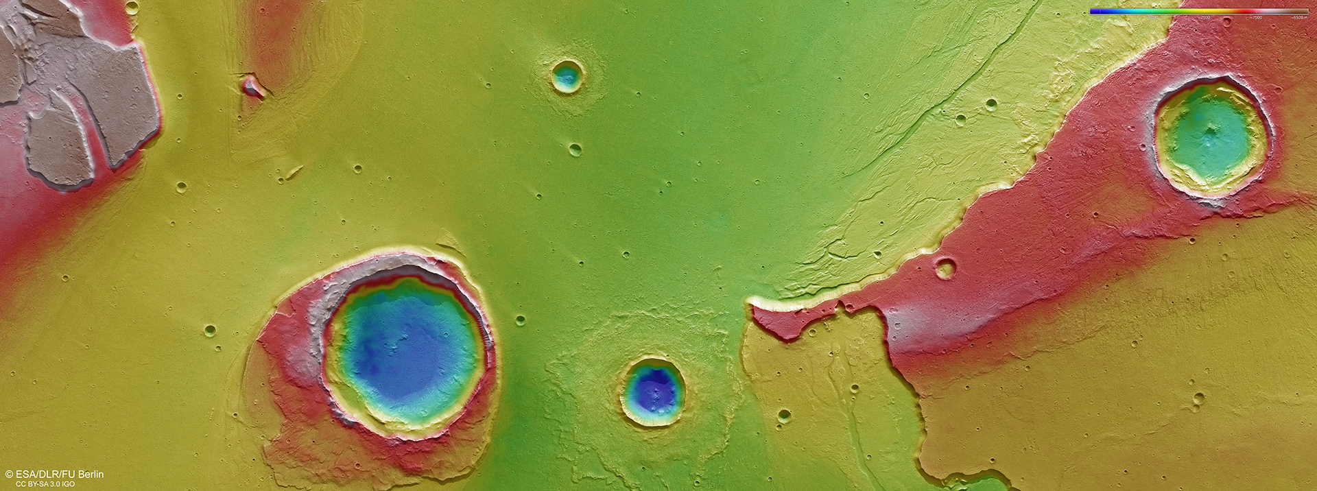
Colour-coded topographic view of the mouth of Kasei Valles, showing the Worcester Crater. Credit: ESA/DLR/FU Berlin.
The Mars Express probe has captured images of this region before. But these latest images, which were snapped n May 25th, 2016, captured the topography of an area that lies at the mouth of the system. Of particular interest was the 25-km-wide Worcester Crater, the remains of an impact that has managed to remain intact despite the erosive force of the mega-flood.
The appearance of this crater and the features around it – which resemble an island – tell us much about the region and its history. For instance, the island has a stepped topography, which is likely the result of its interaction with the flood waters. After the impact threw up material around the crater, moving water pushed it downstream, creating a rigid wall facing towards Kasei Valles and a sloping wall trailing away from it.
The topography of the island is also suggestive of variations in water levels, or possibly different flood episodes. As the water rose and fell, or multiple streams formed over time, the downstream portion of the “island” was affected. There is also the larger crater that appears to the upper right of the image, which sits in a plateau 1 km (0.6 mi) higher than the plains below.
There is a small depression in its center, which would imply that a weaker layer – possibly made of ice – existed under the plateau during the time of impact. This is consistent with the patterns noted in Worcester’s debris blanket, which also suggest the area was rich in water or water-ice during the flooding. The presence of small branch-like channels (aka. dendritic channels) around the plateau are another indication that water levels here varied over time.
Context image shows a region of Mars where Kasei Valles empties into the vast Chryse Planitia. Credit: NASA/MGS/MOLA Science Team
Many smaller craters are also visible in this photo across the mouth of the Kasei Valles region, which also appear to have “tails” of ejected material. This is also true of the crater that sits adjacent to Worchester, who’s debris blanket appears to be largely intact. This would suggest that these craters were formed after the flooding, and any tails that formed were the result of wind.
From all this, it can be concluded that roughly three and a half billion years ago, the mouth of the Kasei Valles region still had water on its surface – possibly still in liquid form but most likely in the form of ice. Volcanic activity – which Mars was still experiencing at the time – then triggered the release of flood waters, which created debris and erosion features throughout the region.
As a result, this latest image manages to capture a preserved record of the geological activity in this region, one which goes back billions of years. And in addition to proving that Mars still had water on its surface, it also confirms that Mars was still experiencing volcanism. It is because of ongoing discoveries like these that the Mars Express mission has been extended several times, the most recent of which extended the mission to end of 2018.
Scientists were able to gauge the rate of water loss on Mars by measuring the ratio of water and HDO from today and 4.3 billion years ago. Credit: Kevin Gill
For years now, scientists have understood that Mars was once a warmer, wetter place. Between terrain features that indicate the presence of rivers and lakes to mineral deposits that appeared to have dissolved in water, there is no shortage of evidence attesting to this “watery” past. However, just how warm and wet the climate was billions of years ago (and since) has been a subject of much debate.
According to a new study from an international team of scientists from the University of Nevada, Las Vegas (UNLV), it seems that Mars may have been a lot wetter than previous estimates gave it credit for. With the help of Berkeley Laboratory, they conducted simulations on a mineral that has been found in Martian meteorites. From this, they determined that Mars may have had a lot more water on its surface than previously thought.
When it comes to studying the Solar System, meteorites are sometimes the only physical evidence available to researchers. This includes Mars, where meteorites recovered from Earth’s surface have helped to shed light on the planet’s geological past and what kinds of processes have shaped its crust. For geoscientists, they are the best means of determining what Mars looked like eons ago.
An artist’s impression of what Mars might have looked like with water, when any potential Martian microbes would have evolved. Credit: ESO/M. Kornmesser
Unfortunately for geoscientists, these meteorites have underdone changes as a result of the cataclysmic force that expelled them from Mars. As Dr. Christopher Adcock, an Assistant Research Professor at with the Dept. of Geoscience at UNLV and the lead author of the study, told Universe Today via email:
“Martian meteorites are pieces of Mars, basically they are our only samples of Mars on Earth until there is a sample return mission. Many of the discoveries we have made about Mars came from studying martian meteorites and wouldn’t be possible without them. Unfortunately, these meteorites have all experienced shock from being ejected of the Martian surface during impacts.”
Of the over 100 Martian meteorites that have been retrieved here on Earth, and range in age from between 4 billion years to 165 million years. They are also believed to have come from only a few regions on Mars, and were likely ejecta created from impact events. And in the course of examining them, scientists have noticed the presence of a calcium phosphate mineral known as merrillite.
As a member of the whitlockite group that is commonly found in Lunar and Martian meteorities, this mineral is known for being anhydrous (i.e. containing no water). As such, researchers have drawn the conclusion that the presence of this minerals indicates that Mars had an arid environment when these rocks were ejected. This is certainly consistent with what Mars looks like today – cold, icy and dry as a bone.
The Mojave Crater on Mars, where some of the Martians meteorites retrieved on Earth are believed to have originated from. Credit: NASA/JPL-Caltech/University of Arizona
For the sake of their study – titled “Shock-Transformation of Whitlockite to Merrillite and the Implications for Meteoritic Phosphate“, which appeared recently in the journal Nature Communications – the international research team considered another possibility. Using a synthetic version of whitlockite, they began conducting shock compression experiments on it designed to simulate the conditions under which meteorites are ejected from Mars.
This consisted of placing the synthetic whitlockite sample inside a projectile, then using a helium gas gun to accelerate it up to speeds of 700 meters per second (2520 km/h or 1500 mph) into a metal plate – thus subjecting it to intense heat and pressure. The sample was then examined using the Berkeley Lab’s Advanced Light Source (ALS) and the Argonne National Laboratory’s Advanced Photon Source (APS) instruments.
“When we analyzed what came out of the capsule, we found a significant amount of the whitlockite had dehydrated to the mineral merrillite,” said Adcock. “Merrillite is found in many meteorites (including Martian). The means it is possible the rocks meteorites are made from originally started life with whitlockite in them in an environment with more water than previously thought. If true, it would indicate more water in the Martian past and the early Solar System.”
Not only does this find raise the “water budget” for Mars in the past, it also raises new questions about Mars’ habitability. In addition to being soluble in water, whitlockite also contains phosphorous – a crucial element for life here on Earth. Combined with recent evidence that shows that liquid water still exists on Mars’ surface – albeit intermittently – this raises new questions about whether or not Mars had life in the past (or even today).
But as Adcock explained, further experiments and evidence will be needed to determine if these results are indicative of a more watery past:
“As far as life goes, our results are very favorable for the possibility – but we need more data. Really we need a sample return mission or we need to go there in person – a human mission. Science is closing in on the answers to a number of big questions about our solar system, life elsewhere, and Mars. But it is difficult work when it all has to be done from far away.”
And sample returns are certainly on the horizon. NASA hopes to conduct the first step in this process with their Mars 2020 Rover, which will collect samples and leave them in a cache for future retrieval. The ESA’s ExoMars rover is expected to make the journey to Mars in the same year, and will also obtain samples as part of a sample-return mission to Earth.
These missions are scheduled to launch the summer of 2020, when the planets will be at their closest again. And with crewed missions to the surface planned for the following decade, we might see the first non-meteorite samples of Mars brought back to Earth for analysis.
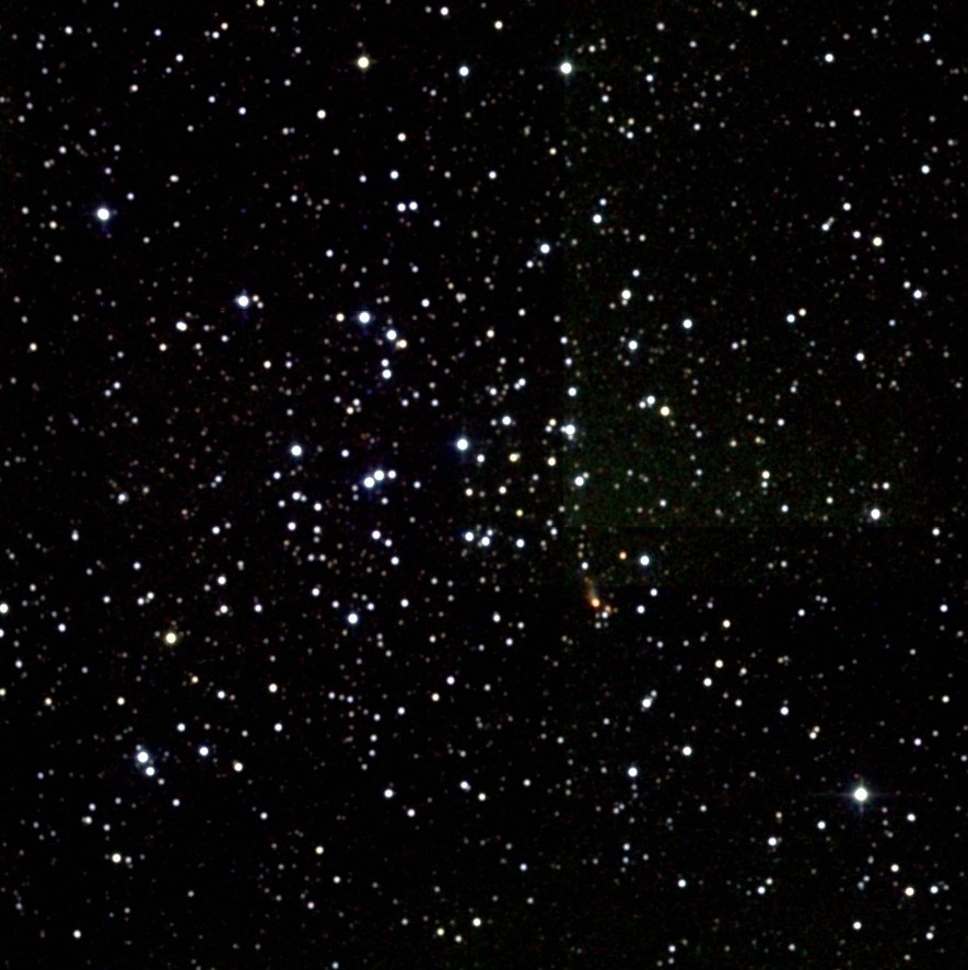
The open star cluster Messier 38, in proximity to Messier 36 and Messier 37. Credit: Wikisky
Welcome back to Messier Monday! In our ongoing tribute to the great Tammy Plotner, we take a look at the Pinweel Cluster, otherwise known as Messier 36. Enjoy!
During the 18th century, famed French astronomer Charles Messier noted the presence of several “nebulous objects” in the night sky. Having originally mistaken them for comets, he began compiling a list of them so that others would not make the same mistake he did. In time, this list (known as the Messier Catalog) would come to include 100 of the most fabulous objects in the night sky.
Included in this list is the open star cluster Messier 36, also known as the Pinwheel Cluster. This cluster is so-named because of its association with the Auriga constellation (aka. “the Charioteer”). Though similar in size and make-up to the Pleiades Cluster (Messier 45), the Pinwheel Cluster is actually ten times farther away from Earth – and one of the most distant of any clusters catalogued by Messier.
What You Are Looking At:
Located a little more than 4000 light years from our solar system, this group of about 60 stars spans across about 14 light years of space. As you are studying it, you’ll notice one star which seems brighter than the rest… With good reason! Its a spectral type B2 and about 360 more luminous than our Sun. Many of the cluster members here are also B-type stars and rapid rotators.
Close-up of the central region of Messier 36. Credit: Wikisky
This means that 25 million year old Messier 36 shares a lot in common with another nearby star cluster, the Pleiades. By taking a deep look at young clusters with stars of varying ages, astronomers are able to how long circumstellar disks may last – giving us a clue as to whether or not planet-forming stars may lay within them.
“We have completed the first systematic and homogeneous survey for circumstellar disks in a sample of young clusters that both span a significant range in age and contain statistically significant numbers of stars whose masses span nearly the entire stellar mass spectrum. Analysis of the combined survey indicates that the cluster disk fraction is initially very high and rapidly decreases with increasing cluster age, such that one-half the stars within the clusters lose their disks in 3 million years. Moreover, these observations yield an overall disk lifetime of ~6 million years in the surveyed cluster sample. This is the timescale for essentially all the stars in a cluster to lose their disks. This should set a meaningful constraint for the planet-building timescale in stellar clusters.”
“The open cluster M36 (NGC 1960), which apparently forms the center of the Aur OB1 association, has been the subject of numerous analyses, and of these the earliest studies are today of historical interest only. NGC 1960 has recently attracted attention as the most likely origin of a massive OB star that exploded about 40,000 yr ago, creating the supernova remnant Simeis 147, an old supernova remnant listed in the catalog compiled at Simeiz by Gaze & Shajn (1952). A pulsar, PSR J0538+2817, has been found near the center of Simeis 147.”
2MASS Atlas Image Mosaic of the open star cluster Messier 36. Credit: NASA/IPAC/Caltech/University of Massachusetts
And the search for planet-building stars within M36 hasn’t stopped yet. The Spitzer Space telescope will also be investigating it, thanks to a proposal made by George Rieke:
“We propose a deep IRAC/MIPS survey of NGC 1960, a ~20 Myr-old massive cluster unexplored in the mid infrared. This cluster is at a key stage in terrestrial planet formation. Our survey will likely detect infrared excess emission from debris disks and transition disks from ~ 100 intermediate-mass (1-3 solar mass) stars. Together with ground-based photometry/spectroscopy of this cluster, proposed observations of 10 Myr-old NGC 6871, scheduled cycle 4 observations of the massive 13 Myr old clusters h and chi Persei, and existing data on NGC 2547 at 30 Myr, this survey will yield robust constraints on the frequency of debris/transition disks as a function of spectral type, age, and cluster environment at a critical age range for planet formation. This survey will provide a benchmark study of the observable signatures of terrestrial planet formation that will inform James Webb Space Telescope observations of planet-forming disks a decade from now.”
History of Observation:
The presence of this awesome star cluster was first recorded by Giovanni Batista Hodierna before 1654 and re-discovered by Le Gentil in 1749. However, it was Charles Messier who took the time to carefully record its position for future generations:
“In the night of September 2 to 3, 1764, I have determined the position of a star cluster in Auriga, near the star Phi of that constellation. With an ordinary refractor of 3 feet and a half, one has difficulty to distinguish these small stars; but when employing a stronger instrument, one sees them very well; they don’t contain between them any nebulosity: their extension is about 9 minutes of arc. I have compared the middle of this cluster with the star Phi Aurigae, and I have determined its position; its right ascension was 80d 11′ 42″, and its declination 34d 8′ 6″ north.”
M36 Open Cluster. Credit: NOAO/AURA/NSF
It would be observed again by Caroline, William and John Herschel who would be the first to note the double star in M36’s center. Although none of their notes are particularly glowing on this awesome star cluster, Admiral Symth does come to the historic rescue!
“A neat double star in a splendid cluster, on the robe below the Waggoner’s left thigh, and near the centre of the Galaxy stream. A [mag] 8 and B 9, both white; in a rich though open splash of stars from the 8th to the 14th magnitudes, with numerous outliers, like the device of a star whose rays are formed by very small stars. This object was registered by M. [Messier] in 1764; and the double star, as H. [John Herschel] remarks, is admirably placed, for future astronomers to ascertain whether there be internal motion in clusters. A line carried from the central star in Orion’s belt, through Zeta Tauri, and continued about 13deg beyond, will reach the cluster, following Phi Aurigae by about two degrees.”
Locating Messier 36:
Locating Messier 36 is relatively easy once you understand the constellation of Auriga. Looking roughly like a pentagon in shape, start by identifying the brightest of these stars – Capella. Due south of it is the second brightest star which shares its border with Beta Tauri, El Nath. By aiming binoculars at El Nath, go north about 1/3 the distance between the two and enjoy all the stars!
You will note two very conspicuous clusters of stars in this area, and so did Le Gentil in 1749. Binoculars will reveal the pair in the same field, as will telescopes using lowest power. The dimmest of these is the M38, and will appear vaguely cruciform in shape. At roughly 4200 light years away, larger aperture will be needed to resolve the 100 or so fainter members. About 2 1/2 degrees to the southeast (about a finger width) you will see the much brighter M36.
The location of M36 in the Auriga constellation. Credit: IAU and Sky and Telescope Magazine (Roger Sinnott & Rick Fienberg)
More easily resolved in binoculars and small scopes, this “jewel box” galactic cluster is quite young and about 100 light years closer. If you continue roughly on the same trajectory about another 4 degrees southeast you will find open cluster M37. This galactic cluster will appear almost nebula-like to binoculars and very small telescopes – but comes to perfect resolution with larger instruments.
While all three open star clusters make fine choices for moonlit or light polluted skies, remember that high sky light means less faint stars which can be resolved – robbing each cluster of some of its beauty. Messier 36 is intermediate brightness of the trio and you’ll quite enjoy its “X” shape and many pairings of stars!
Has the central double changed with time? Why not observe for yourself and see!
Object Name: Messier 36 Alternative Designations: M36, NGC 1960, Pinwheel Cluster Object Type: Galactic Open Star Cluster Constellation: Auriga Right Ascension: 05 : 36.1 (h:m) Declination: +34 : 08 (deg:m) Distance: 4.1 (kly) Visual Brightness: 6.3 (mag) Apparent Dimension: 12.0 (arc min)
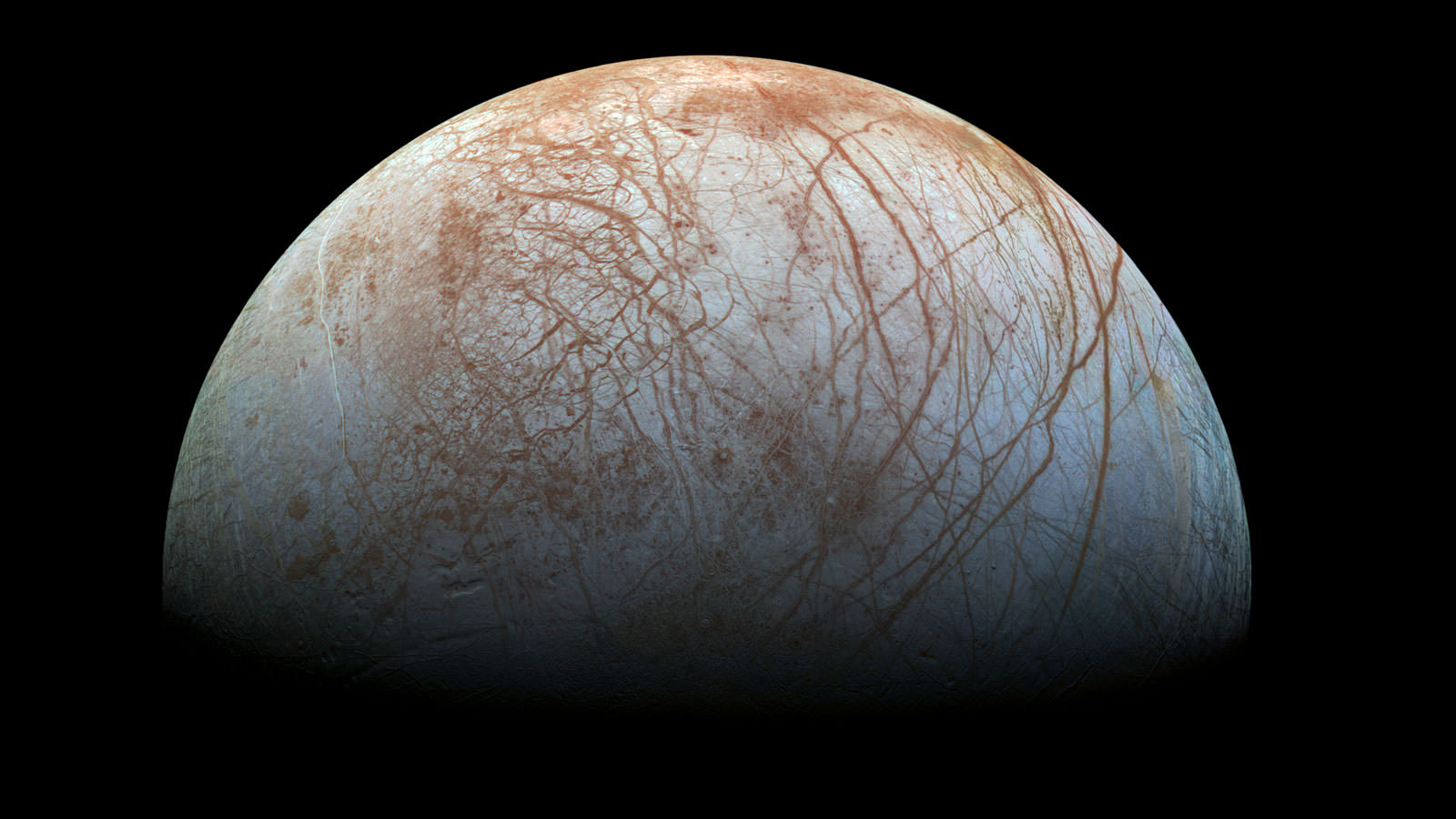
The fascinating surface of Jupiter’s icy moon Europa looms large in this newly-reprocessed color view, made from images taken by NASA's Galileo spacecraft in the late 1990s. This is the color view of Europa from Galileo that shows the largest portion of the moon's surface at the highest resolution. Credits: NASA/JPL-Caltech/SETI Institute
Earlier this week, NASA hosted the “Planetary Science Vision 2050 Workshop” at their headquarters in Washington, DC. Running from Monday to Wednesday – February 27th to March 1st – the purpose of this workshop was to present NASA’s plans for the future of space exploration to the international community. In the course of the many presentations, speeches and panel discussions, many interesting proposals were shared.
Among them were two presentations that outlined NASA’s plan for the exploration of Jupiter’s moon Europa and other icy moons. In the coming decades, NASA hopes to send probes to these moons to investigate the oceans that lie beneath theirs surfaces, which many believe could be home to extra-terrestrial life. With missions to the “ocean worlds” of the Solar System, we may finally come to discover life beyond Earth.
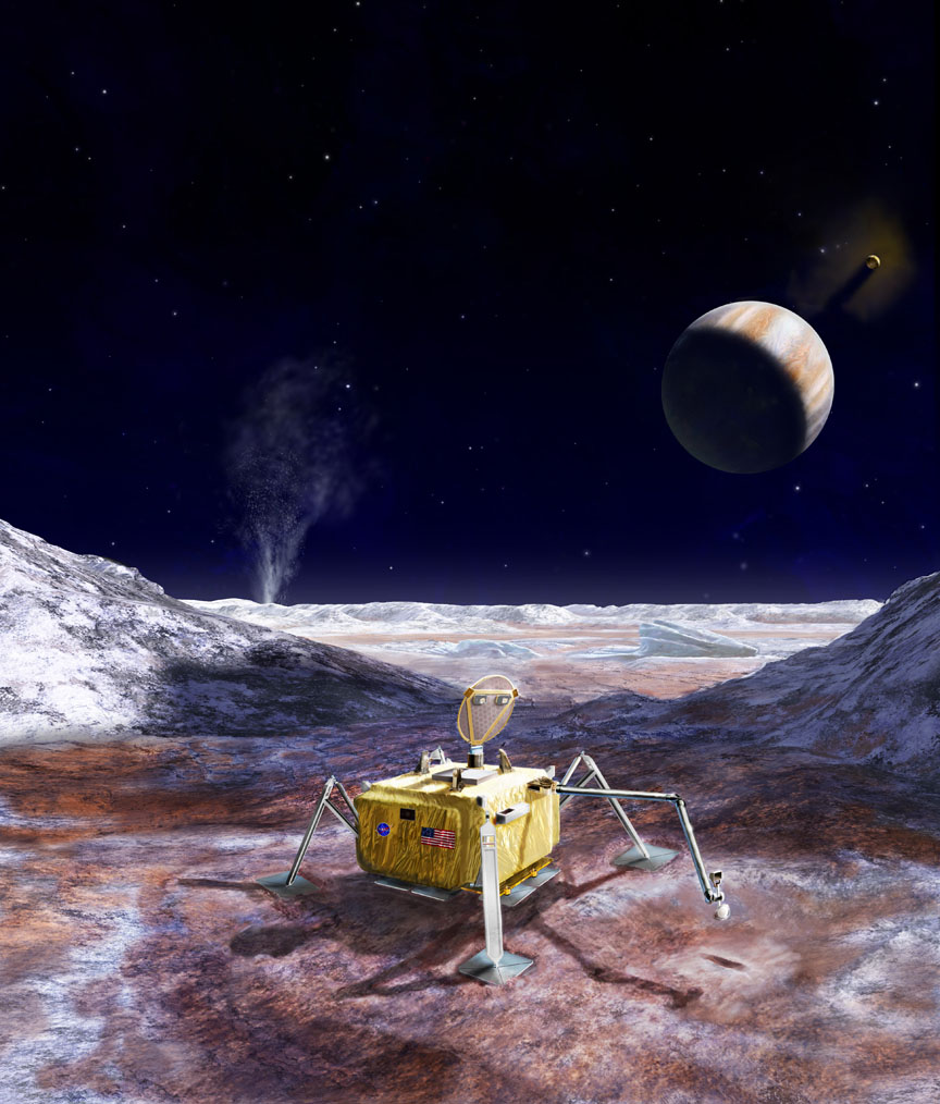
Artist’s rendering of a potential future mission to land a robotic probe on the surface of Jupiter’s moon Europa. Credits: NASA/JPL-Caltech
This report was drafted by NASA’s Planetary Science Division (PSD) in response to a congressional directive to begin a pre-Phase A study to assess the scientific value and engineering design of a Europa lander mission. These studies, which are known as Science Definition Team (SDT) reports, are routinely conducted long before missions are mounted in order to gain an understanding of the types of challenges it will face, and what the payoffs will be.
In addition to being the co-chair of the Science Definition Team, Hand also served as head of the project science team, which included members from the JPL and the California Institute of Technology (Caltech). The report he and his colleagues prepared was finalized and issued to NASA on February 7th, 2017, and outlined several objectives for scientific study.
As was indicated during the course of the presentation, these objectives were threefold. The first would involve searching for biosignatures and signs of life through analyses of Europa’s surface and near-subsurface material. The second would be to conduct in-situ analyses to characterize the composition of non-ice near-subsurface material, and determine the proximity of liquid water and recently-erupted material near the lander’s location.
The third and final goal would be to characterize the surface and subsurface properties and what dynamic processes are responsible for shaping them, in support for future exploration missions. As Hand explained, these objectives are closely intertwined:
“Were biosignatures to be found in the surface material, direct access to, and exploration of, Europa’s ocean and liquid water environments would be a high priority goal for the astrobiological investigation of our Solar System. Europa’s ocean would harbor the potential for the study of an extant ecosystem, likely representing a second, independent origin of life in our own solar system. Subsequent exploration would require robotic vehicles and instrumentation capable of accessing the habitable liquid water regions in Europa to enable the study of the ecosystem and organisms.”
Artist’s impression of a hypothetical ocean cryobot (a robot capable of penetrating water ice) in Europa. Credit: NASA
In other words, if the lander mission detected signs of life within Europa’s ice sheet, and from material churned up from beneath by resurfacing events, then future missions – most likely involving robotic submarines – would definitely be mounted. The report also states that any finds that are indicative of life would mean that planetary protections would be a major requirement for any future mission, to avoid the possibility of contamination.
But of course, Hand also admitted that there is a chance the lander will find no signs of life. If so, Hand indicated that future missions would be tasked with gaining “a better understanding of the fundamental geological and geophysical process on Europa, and how they modulate exchange of material with Europa’s ocean.” On the other hand, he claimed that even a null-result (i.e. no signs of life anywhere) would still be a major scientific find.
Ever since the Voyager probes first detected possible signs of an interior ocean on Europa, scientists have dreamed of the day when a mission might be possible to explore the interior of this mysterious moon. To be able to determine that life does not exist there could no less significant that finding life, in that both would help us learn more about life in our Solar System.
The Science Definition Team’s report will also be the subject of a townhall meeting at the 2017 Lunar and Planetary Science Conference (LPSC) – which will be taking place from March 20th to 24th in The Woodlands, Texas. The second event will be on April 23rd at the Astrobiology Science Conference (AbSciCon) held in Mesa, Arizona. Click here to read the full report.
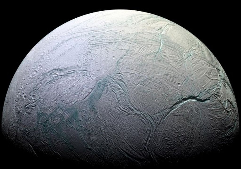
Saturn’s moon Enceladus is another popular destination for proposed missions since it is believed to potentially host extra-terrestrial life. Credit: NASA/JPL/Space Science Institute
The second presentation, titled “Roadmaps to Ocean Worlds” took place later on Monday, Feb. 27th. This presentation was put on by members of the the Roadmaps to Ocean Worlds (ROW) team, which is chaired by Dr. Amandra Hendrix – a senior scientist at the Planetary Science Institute in Tuscon, Arizona – and Dr. Terry Hurford, a research assistant from NASA’s Science and Exploration Directorate (SED).
As a specialist in UV spectroscopy of planetary surfaces, Dr. Hendrix has collaborated with many NASA missions to explore icy bodies in the Solar System – including the Galileo and Cassini probes and the Lunar Reconnaissance Orbiter (LRO). Dr. Hurford, meanwhile, specializes in the geology and geophysics of icy satellites, as well as the effects orbital dynamics and tidal stresses have on their interior structures.
Founded in 2016 by NASA’s Outer Planets Assessment Group (OPAG), ROW was tasked with laying the groundwork for a mission that will explore “ocean worlds” in the search for life elsewhere in the Solar System. During the course of the presentation, Hendrix and Hurford laid out the findings from the ROW report, which was completed in January of 2017.
As they state in this report, “we define an ‘ocean world’ as a body with a current liquid ocean (not necessarily global). All bodies in our solar system that plausibly can have or are known to have an ocean will be considered as part of this document. The Earth is a well-studied ocean world that can be used as a reference (“ground truth”) and point of comparison.”
Dwarf planet Ceres is shown in this false-color renderings, which highlight differences in surface materials. The image is centered on Ceres brightest spots at Occator crater. Credit: NASA/JPL-Caltech/UCLA/MPS/DLR/IDA
By this definition, bodies like Europa, Ganymede,Callisto, and Enceladus would all be viable targets for exploration. These worlds are all known to have subsurface oceans, and there has been compelling evidence in the past few decades that point towards the presence of organic molecules and prebiotic chemistry there as well. Triton, Pluto,Ceres and Dione are all mentioned as candidate ocean worlds based on what we know of them.
Titan also received special mention in the course of the presentation. In addition to having an interior ocean, it has even been ventured that extremophile methanogenic lifeforms could exist on its surface:
“Although Titan possesses a large subsurface ocean, it also has an abundant supply of a wide range of organic species and surface liquids, which are readily accessible and could harbor more exotic forms of life. Furthermore, Titan may have transient surface liquid water such as impact melt pools and fresh cryovolcanic flows in contact with both solid and liquid surface organics. These environments present unique and important locations for investigating prebiotic chemistry, and potentially, the first steps towards life.”
Ultimately, the ROW’s pursuit of life on “ocean worlds” consists of four main goals. These include identifying ocean worlds in the solar system, which would mean determining which of the worlds and candidate worlds would be well-suited to study. The second is to characterize the nature of these oceans, which would include determining the properties of the ice shell and liquid ocean, and what drives fluid motion in them.
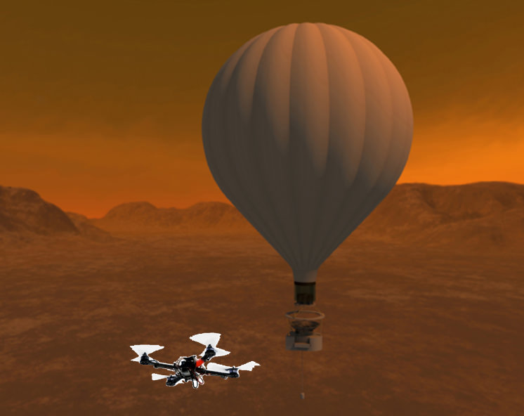
Artist’s conception of the Titan Aerial Daughtercraft on Saturn’s moon Titan. Credit: NASA
The third sub-goal involves determining if these oceans have the necessary energy and prebiotic chemistry to support life. And the fourth and final goal would be to determine how life might exist in them – i.e. whether it takes the form of extremophile bacteria and tiny organisms, or more complex creatures. Hendrix and Hurford also covered the kind of technological advances that will be needed for such missions to happen.
Naturally, any such mission would require the development of power sources and energy storage systems that would be suitable for cryogenic environments. Autonomous systems for pinpoint landing and technologies for aerial or landed mobility would also be needed. Planetary protection technologies would be necessary to prevent contamination, and electronic/mechanical systems that can survive in an ocean world environment too,
While these presentations are merely proposals of what could happen in the coming decades, they are still exciting to hear about. If nothing else, they show how NASA and other space agencies are actively collaborating with scientific institutions around the world to push the boundaries of knowledge and exploration. And in the coming decades, they hope to make some substantial leaps.
If all goes well, and exploration missions to Europa and other icy moons are allowed to go forward, the benefits could be immeasurable. In addition to the possibility of finding life beyond Earth, we will come to learn a great deal about our Solar System, and no doubt learn something more about humanity’s place in the cosmos.
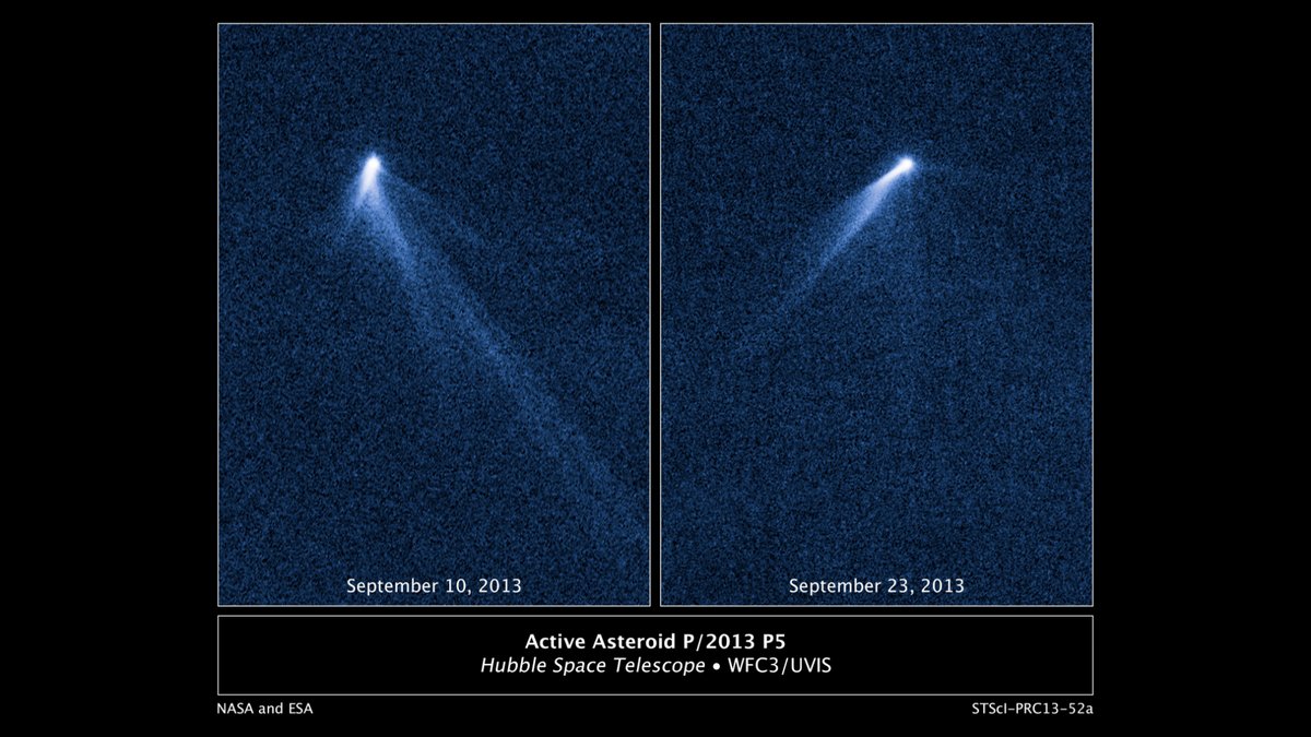
Images from the Hubble Space Telescope of activated asteroid P/2013P5 where the dust tail can be seen. Source: NASA/ESA.
In the 18th and 19th centuries, astronomers made some profound discoveries about asteroids and comets within our Solar System. From discerning the true nature of their orbits to detecting countless small objects in the Main Asteroid Belt, these discoveries would inform much of our modern understanding of these bodies.
A general rule about comets and asteroids is that whereas the former develop comas or tails as they undergo temperature changes, the latter do not. However, a recent discovery by an international group of researchers has presented another exception to this rule. After viewing a parent asteroid in the Main Belt that split into a pair, they noted that both fragments formed tails of their own.
The reason asteroids do not do behave like comets has a lot to do with where they are situated. Located predominantly in the Main Belt, these bodies have relatively circular orbits around the Sun and do not experience much in the way of temperature changes. As a result, they do not form tails (or halos), which are created when volatile compounds (i.e. nitrogen, hydrogen, carbon dioxide, methane, etc.) sublimate and form clouds of gas.
Images of the P/2016 J1 asteroid pair taken on May 15th, 2016. They show a central region, the asteroid, and a diffuse blot corresponding to the dust tail. Credit: IAA
As astronomical phenomena go, asteroid pairs are quite common. They are created when an asteroid breaks in two, which can be the result of excess rotational speed, impact with another body, or because of the destabilization of binary systems (i.e. asteroid that orbit each other). Once this happens, these two bodies will orbit the Sun rather than being gravitational bound to each other, and progressively drift farther apart.
However, when monitoring the asteroid P/2016 J1, an international team from the Institute of Astrophysics in Andalusia (IAA-CSIC) noticed something interesting. Apparently, both fragments in the pair had become “activated” – that is to say, they had formed tails. As Fernando Moreno, a researcher at IAA-CSIC who led the project, said in an Institute press release:
“Both fragments are activated, i.e., they display dust structures similar to comets. This is the first time we observe an asteroid pair with simultaneous activity… In all likelihood, the dust emission is due to the sublimation of ice that was left exposed after the fragmentation.”
While this is not the first instance where asteroids proved to be an exception to the rule and began forming clouds of sublimated gas around them, this is the first time it was observed happening with an asteroid pair. And it seems that the formation of this tail was in response to the breakup, which is believed to have happened six years ago, during the previous orbit of the asteroid.
An artist’s conception of two tidally locked objects orbiting the Sun from afar (2010 WG9). Credit: zmescience
In 2016, the research team used the Great Telescope of the Canary Islands (GTC) on the island of La Palma and the Canada-France-Hawaii Telescope (CFHT) at Mauna Kea to confirm that the asteroid had formed a pair. Further analysis revealed that the asteroids were activated between the end of 2015 and the beginning of 2016, when they reached the closest point in their orbit with the Sun (perihelion).
This analysis also revealed that the fragmentation of the asteroid and the bout of activity were unrelated. In other words, the sublimation has happened since the breakup and was not the cause of it. Because of this, these objects are quite unique as far as Solar System bodies go.
Not only are they two more exceptions to the rule governing comets and asteroids (there are only about twenty known cases of asteroids forming tales), the timing of their breakup also means that they are the youngest asteroid pair in the Solar System to date. Not bad for a bunch of rocks!
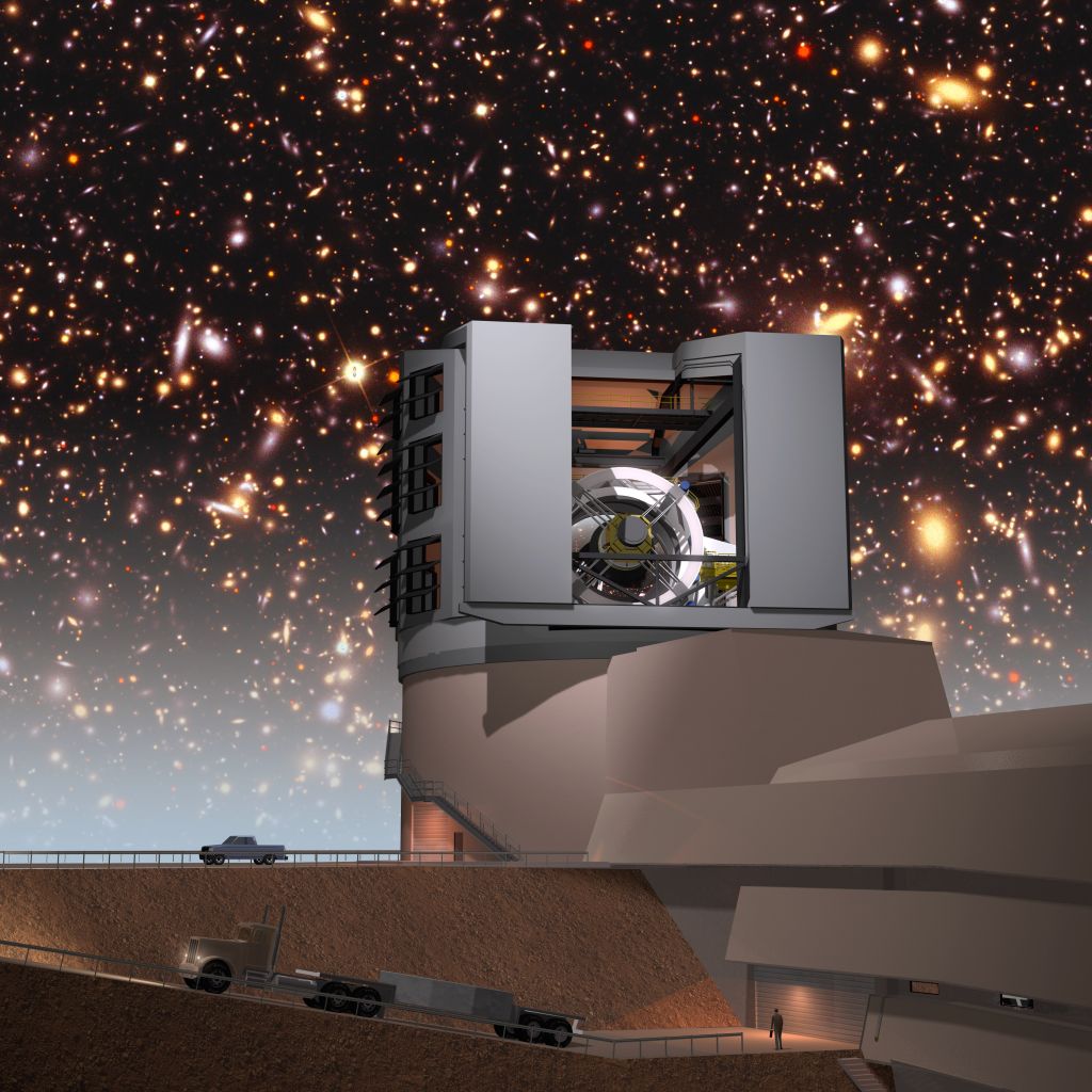
An artist's illustration of the Large Synoptic Survey Telescope with a simulated night sky. The team hopes to use the LSST to further refine their search for hard-surface supermassive objects. Image: Todd Mason, Mason Productions Inc. / LSST Corporation
We humans have an insatiable hunger to understand the Universe. As Carl Sagan said, “Understanding is Ecstasy.” But to understand the Universe, we need better and better ways to observe it. And that means one thing: big, huge, enormous telescopes.
In this series we’ll look at 6 of the world’s Super Telescopes:
While the world’s other Super Telescopes rely on huge mirrors to do their work, the LSST is different. It’s a huge panoramic camera that will create an enormous moving image of the Universe. And its work will be guided by three words: wide, deep, and fast.
While other telescopes capture static images, the LSST will capture richly detailed images of the entire available night sky, over and over. This will allow astronomers to basically “watch” the movement of objects in the sky, night after night. And the imagery will be available to anyone.
The LSST is being built by a group of institutions in the US, and even got some money from Bill Gates. It will be situated atop Cerro Pachon, a peak in Northern Chile. The Gemini South and Southern Astrophysical Research Telescopes are also situated there.
The Camera Inside the ‘Scope
At the heart of the LSST is its enormous digital camera. It weighs over three tons, and the sensor is segmented in a similar way that other Super Telescopes have segmented mirrors. The LSST’s camera is made up of 189 segments, which together create a camera sensor about 2 ft. in diameter, behind a lens that is over 5 ft. in diameter.
Each image that the LSST captures is 40 times larger than the full moon, and will measure 3.2 gigapixels. The camera will capture one of these wide-field images every 20 seconds, all night long. Every few nights, the LSST will give us an image of the entire available night sky, and it will do that for 10 years.
“The LSST survey will open a movie-like window on objects that change brightness, or move, on timescales ranging from 10 seconds to 10 years.” – LSST: FROM SCIENCE DRIVERS TO REFERENCE DESIGN AND ANTICIPATED DATA PRODUCTS
The LSST will capture a vast, movie-like image of over 40 billion objects. This will range from distant, enormous galaxies all the way down to Potentially Hazardous Objects as small as 140 meters in diameter.
The primary-tertiay mirror at its construction facility. Image: LSST
There’s a whole other side to the LSST which is a little more challenging. We get the idea of an in-depth, moving, detailed image of the sky. That’s intuitively easy to engage with. But there’s another side, the data mining challenge.
The Data Challenge
The whole endeavour will create an enormous amount of data. Over 15 terabytes will have to be processed every night. Over its 10 year lifespan, it will capture 60 petabytes of data.
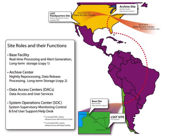
Once data is captured by the LSST, it will travel via two dedicated 40 GB lines to the Data Processing and Archive Center. That Center is a super-computing facility that will manage all the data and make it available to users. But when it comes to handling the data, that’s just the tip of the iceberg.
“LSST is a new way to observe, and gaining knowledge from the Big Data LSST delivers is indeed a challenge.” – Suzanne H. Jacoby, LSST
The sheer amount of data created by the LSST is a challenge that the team behind it saw coming. They knew they would have to build the capacity of the scientific community in advance, in order to get the most out of the LSST.
Handling all of the data from the LSST requires its own infrastructure. Image: LSST
As Suzanne Jacoby, from the LSST team, told Universe today, “To prepare the science community for LSST Operations, the LSST Corporation has undertaken an “Enabling Science” effort which funds the LSST Data Science Fellowship Program (DSFP). This two-year program is designed to supplement existing graduate school curriculum and explores topics including statistics, machine learning, information theory, and scalable programming.”
The Science
The Nature of Dark Matter and Understanding Dark Energy
Contributing to our understanding Dark Energy and Dark Matter is a goal of all of the Super Telescopes. The LSST will map several billion galaxies through time and space. It will help us understand how Dark Energy behaves over time, and how Dark Matter affects the development of cosmic structure.
Cataloging the Solar System
The raw imaging power of the LSST will be a game-changer for mapping and cataloguing our Solar System. It’s thought that the LSST could detect between 60-90% of all potentially hazardous asteroids (PHAs) larger than 140 meters in diameter, as far away as the main asteroid belt. This will not only contribute to NASA’s goal of identifying threats to Earth posed by asteroids, but will help us understand how planets formed and how our Solar System evolved.
Exploring the Changing Sky
The repeated imaging of the night sky, at great depth and with excellent image quality, should tell us a lot about supernovae, variable stars, and possible other events we haven’t even discovered yet. There are always surprising results whenever we build a new telescope or send a probe to a new destination. The LSST will probably be no different.
Milky Way Structure & Formation
The LSST will give us an unprecedented look at the Milky Way. It will survey over half of the sky, and will do so repeatedly. Hundreds of times, in fact. The end result will be an enormously detailed look at the motion of millions of stars in our galaxy.
Open Access
Perhaps the best part of the whole LSST project is that the all of the data will be available to everyone. Anyone with a computer and an internet connection will be able to access LSST’s movie of the Universe. It’s warm and fuzzy, to be sure, to have the results of large science endeavours like this available to anyone. But there’s more to it. The LSST team suspects that the majority of the discoveries resulting from its rich data will come from unaffiliated astronomers, students, and even amateurs.
It was designed from the ground up in this way, and there will be no delay or proprietary barriers when it comes to public data access. In fact, Google has signed on as a partner with LSST because of the desire for public access to the data. We’ve seen what Google has done with Google Earth and Google Sky. What will they come up with for Google LSST?
The Sloan Digital Sky Survey (SDSS), a kind of predecessor to the LSST, was modelled in the same way. All of its data was available to astronomers not affiliated with it, and out of over 6000 papers that refer to SDSS data, the large majority of them were published by astronomers not affiliated with SDSS.
First Light
We’ll have to wait a while for all of this to come our way, though. First light for the LSST won’t be until 2021, and it will begin its 10 year run in 2022. At that time, be ready for a whole new look at our Universe. The LSST will be a game-changer.
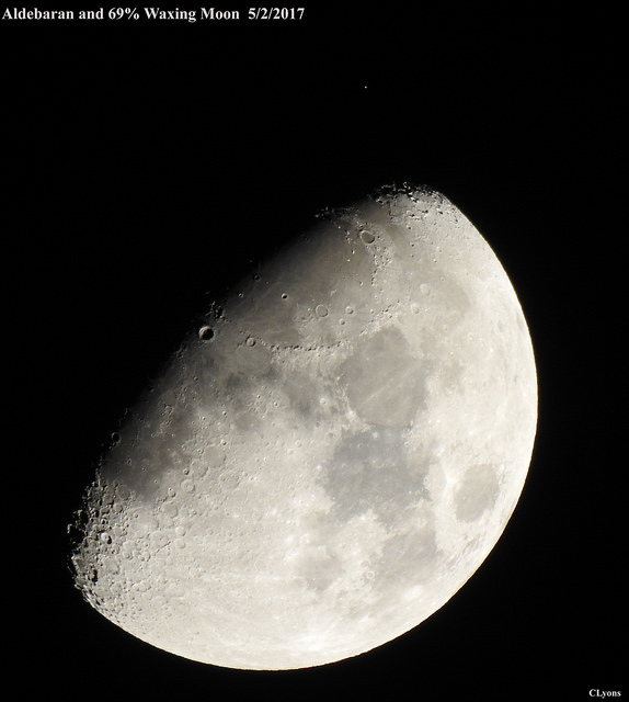
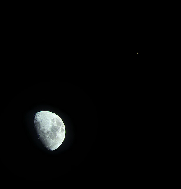
The Moon nearing Aldebaran on February 5th, 2017. Image credit and copyright: Chris Lyons.
The Moon nearing Aldebaran on February 5th, 2017. Image credit and copyright: Chris Lyons.
Ever watch the Moon cover up a star? There’s a great chance to see just such an event this coming weekend, when the waxing gibbous Moon occults (passes in front of) the bright star Aldebaran for much of North America on Saturday night, March 4th.
Shining at magnitude +0.85, Aldebaran is the brightest star that lies along the Moon’s path in the current epoch, and is one of four +1st magnitude stars that the Moon can occult. The other three are Regulus, Antares and Spica. This is the 29th in a series of 49 occultations of Aldebaran worldwide spanning from January 29th, 2015 to September 3rd, 2018, meaning Aldebaran hides behind the Moon once every lunation as it crosses through the constellation Taurus and the Hyades open star cluster in 2017. Like eclipses belonging to the same saros cycle, successive occultations of bright stars shift westward by about 120 degrees westward longitude and slowly drift to the north. Europe saw last month’s occultation of Aldebaran, and Asia is up next month on April 1st.
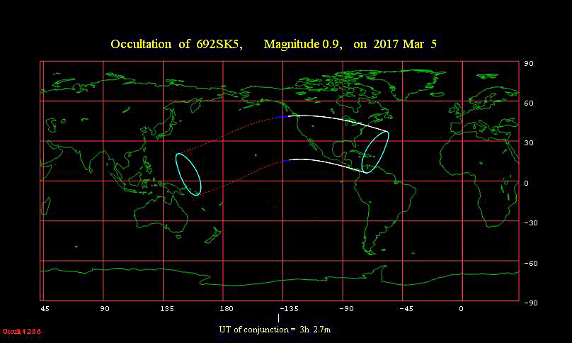
The occultation footprint for Saturday night’s event. Credit: Occult 4.2 software.
All of the contiguous ‘lower 48 states’ except northern New England see Saturday night’s occultation, and under dark skies, to boot. It’s a close miss for Canada. Mexico, central America and the Caribbean will also witness the event under dark skies. Hawaii will see the event under daytime skies. We can attest that this is indeed possible using binocs or a telescope, as we caught Aldebaran near the daytime Moon during last month’s event.
Occultations give us a chance to see a split second magic act, in a Universe that often unfolds over eons and epochs. The motion you’re seeing is mostly that of the Moon, and to a lesser extent, that of the Earth as the star abruptly ‘winks out’.
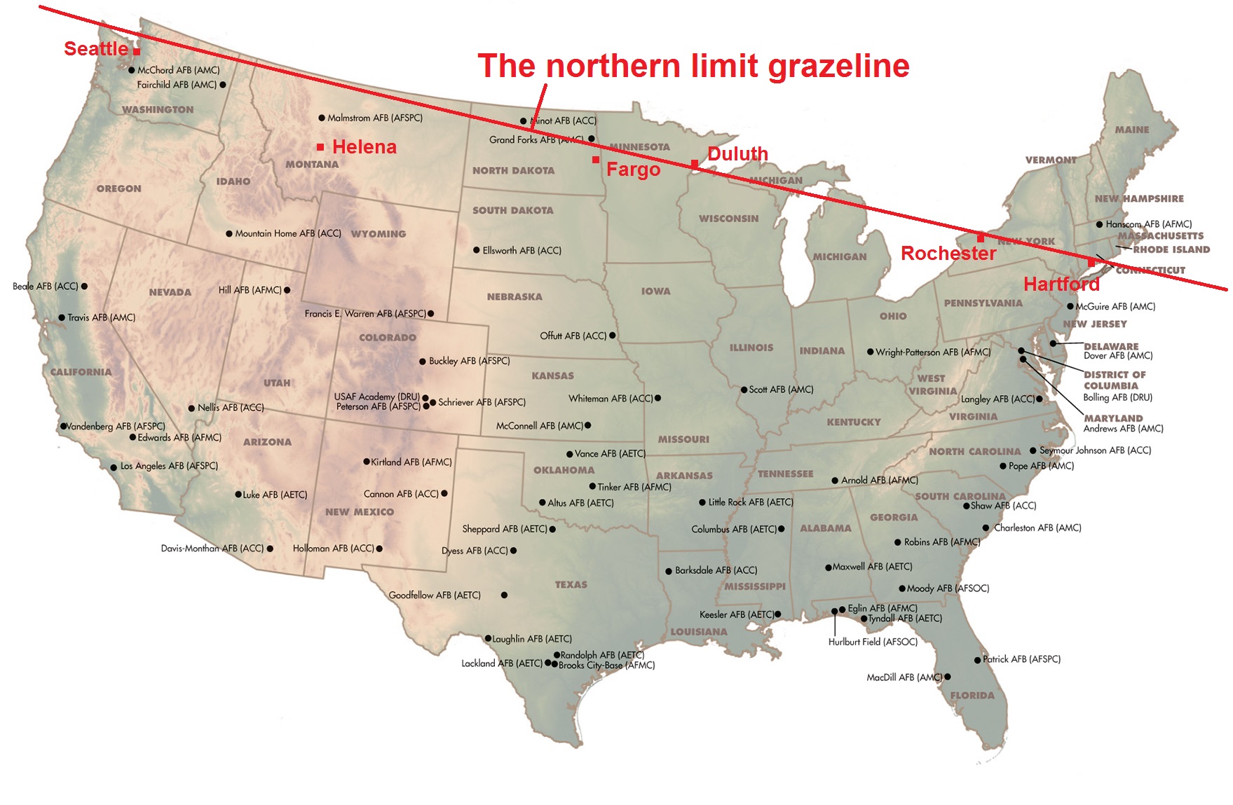
Observers in northern tier states might witness an additional spectacle, as Aldebaran grazes the northern limb of the Moon. This can make for an unforgettable sight, as the star successively winks in at out from behind lunar peaks and valleys. The graze line for Saturday night follows the U.S./Canadian border from Washington state, Idaho and Montana, then transects North Dakota, Minnesota just below Duluth and northern Wisconsin, Michigan and New York and Connecticut. Brad Timerson over at the international Occultation Timing Association has a good page set up for the circumstances for the grazing event, and the IOTA has a page detailing ingress (start) and egress times for the event for specific cities.
The northern limit grazeline for Saturday night’s occultation. Credit: USAF/Wikimedia Commons/Dave Dickinson
You’ll be able to see the occultation of Aldebaran with the unaided eye, no telescope over binocular needed, though it will be fun to follow along with optics as well. The ingress along the leading dark limb of the Moon is always more dramatic, while reemergence on the bright limb is a more subtle affair.
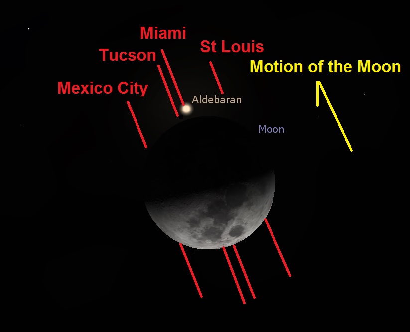
The path of the occultation for select cities. Credit: Stellarium.
A simple video aimed afocally through a telescope eyepiece can easily capture the event. We like to run WWV radio on AM shortwave in the background while video recording so as to get a good time hack of the event on audio. Finally, set up early, watch those battery levels in the frigid March night, and be sure to balance out your exposure times to capture both Aldebaran and the dazzling limb of the Moon.
Can you see it? The Moon paired with Aldebaran on February 5th. Image credit and copyright: Lucca Ruggiero.
Anyone Live-casting the event? It’ll be a tough one low to the horizon here in central Florida, but a livestream would certainly be possible for folks westward with Aldebaran and the Moon high in the sky. Let us know of any planned webcasts, and we’ll promote accordingly.
The Moon also occults several other bright stars this week, leading up to an occultation of Regulus on March 10th favoring the southern Atlantic. Read all about occultations, eclipses, comets and more in our free e-book, 101 Astronomical Events for 2017 from Universe Today.
Don’t miss Saturday night’s stunning occultation, and let us know of your tales of astronomical tribulation and triumph.
-Send those astro-images in to Universe Today’s Flickr forum, and you might just see ’em featured here in a future article.