A Novel Concept For Braking Breakthrough Starshot

Artist concept of lightsail craft approaching the potentially habitable exoplanet Proxima b. Credit: PHL @ UPR Arecibo

In April of 2016, Russian billionaire Yuri Milner announced the creation of Breakthrough Starshot. As part of his non-profit scientific organization (known as Breakthrough Initiatives), the purpose of Starshot was to design a lightsail nanocraft that would be capable of reaching the nearest star system – Alpha Centauri (aka. Rigel Kentaurus) – within our lifetime.

Since its inception, the scientists and engineers behind the Starshot concept have sought to address the challenges that such a mission would face. Similarly, there have been many in the scientific community who have also made suggestions as to how such a concept could work. The latest comes from the Max Planck Institute for Solar System Research, where two researchers came up with a novel way of slowing the craft down once it reaches its destination.

To recap, the Starshot concept involves a small, gram-scale nanocraft being towed by a lightsail. Using a ground-based laser array, this lightsail would be accelerated to a velocity of about 60,000 km/s (37,282 mps) – or 20% the speed of light. At this speed, the nanocraft would be able to reach the closest star system to our own – Alpha Centauri, located 4.37 light-years away – in just 20 years time.

Project Starshot, an initiative sponsored by the Breakthrough Foundation, is intended to be humanity’s first interstellar voyage. Credit: breakthroughinitiatives.org

Naturally, this presents a number of technical challenges – which include the possibility of a collision with interstellar dust, the proper shape of the lightsail, and the sheer energy requirements for powering the laser array. But equally important is the idea of how such a craft would slow down once it reached its destination. With no lasers at the other end to apply breaking energy, how would the craft slow down enough to begin studying the system?

It was this very question that René Heller and Michael Hippke chose to address in their study, “Deceleration of high-velocity interstellar photon sails into bound orbits at Alpha Centauri“. Heller is an astrophysicts who is currently assisting the ESA with its preparations for the upcoming PLAnetary Transits and Oscillations of stars (PLATO) mission – an exoplanet hunter being deployed as part of their Cosmic Vision program.

With the help IT specialist Michael Hippke, the two considered what would be needed for interstellar mission to reach Alpha Centauri, and provide good scientific returns upon its arrival. This would require that braking maneuvers be conducted once it arrived so the the spacecraft would not overshoot the system in the blink of an eye. As they state in their study:

“Although such an interstellar probe could reach Proxima 20 years after launch, without propellant to slow it down it would traverse the system within hours. Here we demonstrate how the stellar photon pressures of the stellar triple Alpha Cen A, B, and C (Proxima) can be used together with gravity assists to decelerate incoming solar sails from Earth.”

The projected path a lightsail mission to Alpha Centauri could take, which would allow it to detour to Proxima Centauri. Credit: PHL @ UPR Arecibo.

For the sake of their calculations, Heller and Hippke estimated that the craft would weigh less than 100 grams (3.5 ounces), and would be mounted on a sail measuring 100,000 m² (1,076,391 square foot) in surface area. Once these were complete, Hippke adapted them into a series of computer simulations. Based on their results, they proposed an entirely new mission concept that do away with the need for lasers entirely.

In essence, their revised concept called for an Autonomous Active Sail (AAS) craft that would provide for its own propulsion and stopping power. This craft would deploy its sail while in the Solar System and use the Sun’s solar wind to accelerate it to high speeds. Once it reached the Alpha Centauri System, it would redeploy its sail so that incoming radiation from Alpha Centauri A and B would have the effect of slowing it down.

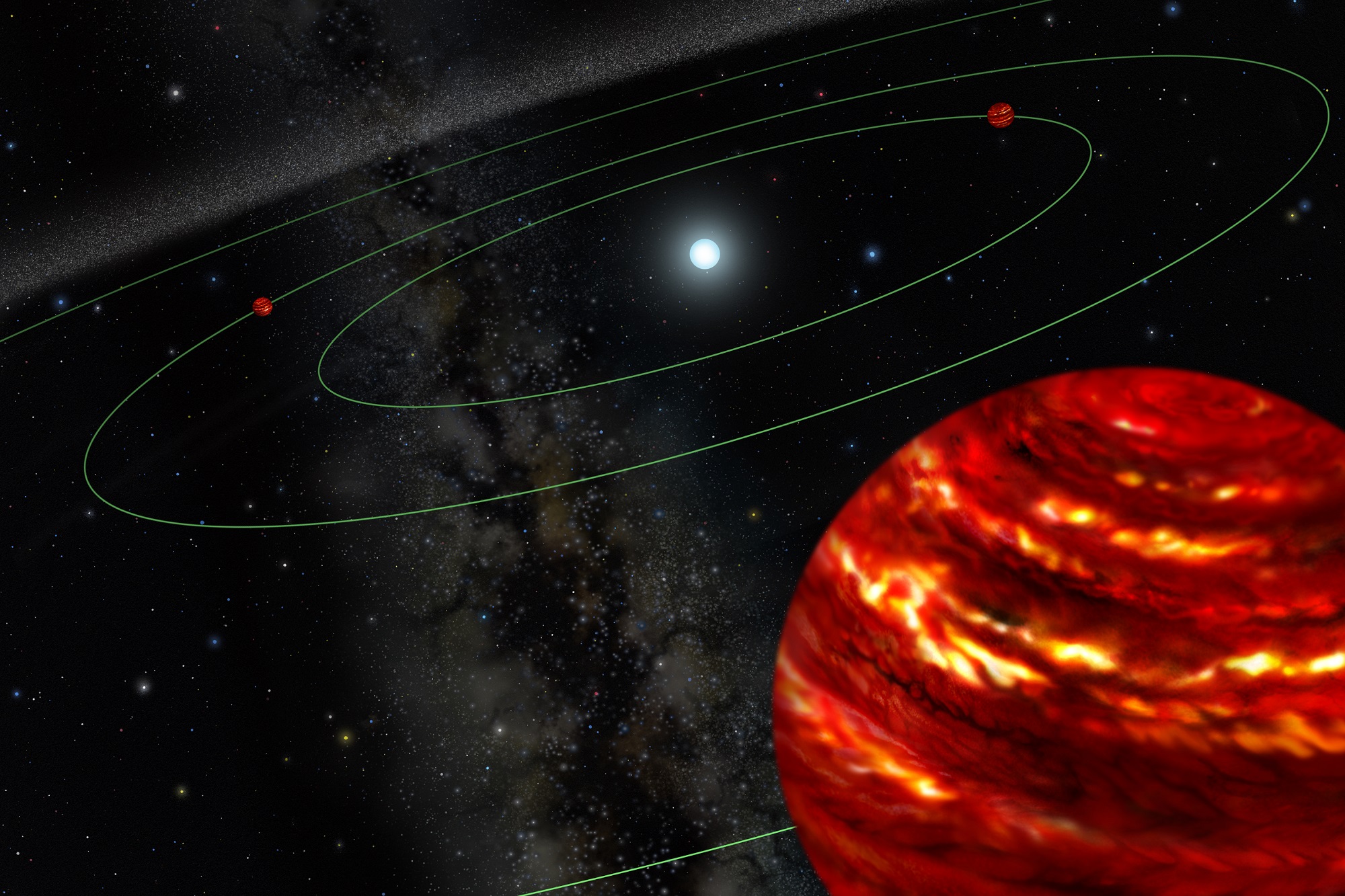
An added bonus of this proposed maneuver is that the craft, once it had been decelerated to the point that it could effectively explore the Alpha Centauri system, could then use a gravity assist from these stars to reroute itself towards Proxima Centauri. Once there, it could conduct the first up-close exploration of Proxima b – the closest exoplanet to Earth – and determine what its atmospheric and surface conditions are like.

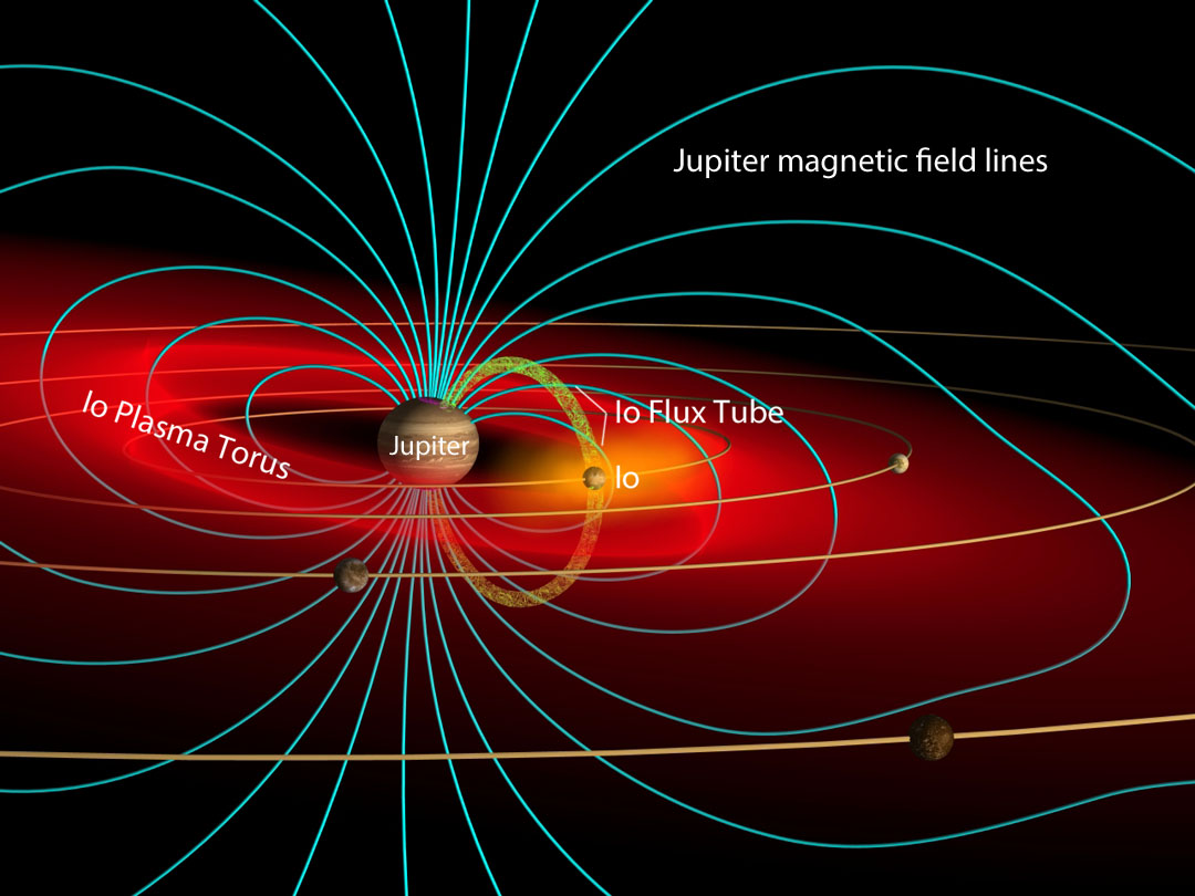
Since the existence of this planet was first announced by the European Southern Observatory back in August of 2016, there has been much speculation about whether or not it could be habitable. Having a mission that could examine it to check for the telltale markers – a viable atmosphere, a magnetosphere, and liquid water on the surface – would surely settle that debate.

As Heller explained in a press release from the Max Planck Institute, this concept presents quite a few advantages, but comes with its share of trade offs – not the least of which is the time it would take to get to Alpha Centauri. “Our new mission concept could yield a high scientific return, but only the grandchildren of our grandchildren would receive it,” he said. “Starshot, on the other hand, works on a timescale of decades and could be realized in one generation. So we might have identified a longterm, follow-up concept for Starshot.”

At present, Heller and Hippke are discussing their concept with Breakthrough Starshot to see if it would be viable. One individual who has looked over their work is Professor Avi Loeb, the Frank B. Baird Jr. Professor of Science at Harvard University, and the chairman of the Breakthrough Foundation’s Advisory Board. As he told Universe Today via email, the concept put forth by Heller and Hippke is worthy of consideration, but has its limitations:

“If it is possible to slow down a spacecraft by starlight (and gravitational assist), then it is also possible to launch it in the first place by the same forces… If so, why is the recently announced Breakthrough Starshot project using a laser and not Sunlight to propel our spacecraft? The answer is that our envisioned laser array can push the sail with an energy flux that is a million times larger than the local solar flux.

“In using starlight to reach relativistic speeds, one must use an extremely thin sail. In the new paper, Heller and Hippke consider the example of a milligram instead of a gram-scale sail. For a sail of area ten square meters (as envisioned in our Starshot concept study), the thickness of their sail must be only a few atoms. Such a surface is orders of magnitude thinner than the wavelength of light that it aims to reflect, and so its reflectivity would be low. It does not appear feasible to reduce the weight by so many orders of magnitude and yet maintain the rigidity and reflectivity of the sail material.

“The main constraint in defining the Starshot concept was to visit Alpha Centauri within our lifetime. Extending the travel time beyond the lifetime of a human, as advocated in this paper, would make it less appealing to the people involved. Also, one should keep in mind that the sail must be accompanied by electronics which will add significantly to its weight.”

In short, if time is not a factor, we can envision that our first attempts to reach another Solar System may indeed involve an AAS being propelled and slowed down by solar wind. But if we’re willing to wait centuries for such a mission to be completed, we might also consider sending rockets with conventional engines (possibly even crewed ones) to Alpha Centauri.

But if we are intent on getting there within our own lifetimes, then a laser-driven sail or something similar will have be the way to go. Humanity has spent over half a century exploring what’s in our own backyard, and some of us are impatient to see what’s next door!

Further Reading: Max Planck Institute, ArXiv

Superbowl Smackdown: Watch the Moon Occult Aldebaran on Sunday

Daytime Aldebaran
Can you see it? Dave Walker accidentally (!) caught Aldebaran near the daytime Moon on October 19th, 2016. Image credit and copyright: Dave Walker
Daytime Aldebaran
Can you see it? Dave Walker accidentally (!) caught Aldebaran near the daytime Moon on October 19th, 2016. Image credit and copyright: Dave Walker

Author’s note: This Superbowl Sunday event and 101 more like it are featured in our latest free e-book, 101 Astronomical Events for 2017, out now from Universe Today.

Sure, this Superbowl Sunday brings with it the promise of sacks, fumbles and tackles… but have you ever seen the Moon run down a star in the end zone? Just such an event, referred to as an occultation, happens this weekend for folks living around the Mediterranean and — just maybe for some sharp-eyed, telescope-owning observers based around the Caribbean region — this coming weekend.

Update: be sure to watch this Sunday’s occultation of Aldebaran by the Moon courtesy of Gianluca Masi and the Virtual Telescope Project live starting at 22:00 UT/5:00 PM EST:

Live starting at 22:00 UT. Credit: The Virtual Telescope Project

We’re talking about Sunday’s occultation of the bright star Aldebaran by the 64% illuminated waxing gibbous Moon. This is the 2nd occultation of Aldebaran by the Moon for 2017 and the 28th of the current ongoing cycle of 49 spanning from January 29th, 2015 to September 3rd, 2018. The Moon actually occults Aldebaran and Regulus once for every lunation in 2017. We won’t have another year featuring the occultations of two +1st magnitude stars (Spica and Antares) again until 2024.

Occultation footprint
The footprint for the February 5th occultation of Aldebaran by the Moon. The broken lines show where the occultation occurs during daytime, and the solid lines denote where the occultation occurs under dark skies. Image credit: occult 4.2.

The event occurs under dark skies for observers based around the Mediterranean and under daytime afternoon skies for folks in central America, the Caribbean, northern South America and the Florida peninsula, including Astroguyz HQ based in Spring Hill, just north of the Tampa Bay area. We’ve managed to spy Aldebaran near the daytime Moon while the Sun was still above the horizon using binocs, and can attest that the +1st magnitude star is indeed visible, if you know exactly where to look for it.

Note that, like solar eclipses belonging to the same saros cycle, occultations of Aldebaran in the ongoing cycle drift north and westward from one to the next, to the tune of about 120 degrees longitude. Though most of North America sits this one out, we do get a front row seat for next lunation’s occultation of Aldebaran on the evening of March 4/5th. The next one is the best bright star occultation of Aldebaran by the Moon for North America in 2017. And be sure to check out the Moon this Sunday evening after the big game, and note Aldebaran hanging just off of its bright limb.

Moon motion
No, the wind is not shaking the ‘scope… Sharin Ahmad chronicled the motion of the Moon past Aldebaran from Kuala Lumpur, Malaysia last month. Image credit and copyright: Shahrin Ahmad (@shahgazer)

The ref will have a close call to make for this one. The northern grazeline in Florida might make this an especially interesting event to watch, though it’ll be challenge, as the occultation occurs in the afternoon under daylight skies. This crosses right along near the cities of Jacksonville and Gainsville. Clear, deep blue high contrast skies are key, and we’ll be watching from Astroguyz HQ north of Tampa Bay during this event.

The northern grazeline across the Florida peninsula for Sunday’s ‘big game’. Credit: Dave Dickinson.

Here are some key times from the occultation zone (noted in Universal Time):

Tampa, Florida

Ingress: 20:08 UT/Moon altitude: 23 degrees

Egress: 20:34 UT/Moon altitude: 29 degrees

Bogota, Columbia

Ingress: 19:34 UT/ Moon Altitude: 49 degrees

Egress: 20:29 UT/ Moon altitude: 31 degrees

The view from Jimena de la Frontera Spain just before the occultation. Credit: Stellarium.

Rome, Italy

Ingress: 20:21 UT/Moon altitude: 37 degrees

Egress: 23:12 UT/ Moon altitude: 28 degrees

Tel Aviv, Israel

Ingress: 22:39 UT/Moon altitude: 16 degrees

Egress: 23:29 UT/Moon altitude: 5 degrees

Casablanca, Morocco

Ingress: 21:49 UT/ Moon altitude: 61 degrees

Egress: 23:07 UT/ Moon altitude: 45 degrees

Note that this occultation spans five continents, a truly worldwide event. The International Occultation Timing Association (IOTA) maintains a page with an extensive list of times for cities worldwide. Note that when the Moon tackles Aldebaran, its also crossing the scrimmage line of the Hyades open cluster, so expect numerous occultations of fainter stars worldwide as well.

Aldebaran is the brightest star along the Moon’s path in our current epoch, along with runner-ups Spica, Regulus and Antares. Though Aldebaran is 1.5 times the mass of our Sun, it’s also 65 light years away, and only appears 20 milliarcseconds (mas) in size, about the equivalent of a 40 meter diameter crater from the distance of the Moon. Still, you might just notice a brief pause as Aldebaran fades then winks out on the dark limb of the Moon, a tiny hitch betraying its diminutive angular size.

And the clockwork gears of that biggest game of all, the Universe, grind on. Don’t miss this first big ticket astronomical event for February 2017, coming to a sky above you. Next up, we’ll watching out for another bright star occultation, two eclipses, and the close passage of a comet near the Earth.

Stay tuned!

What is the Weather like on Mars?

Image taken by the Viking 1 orbiter in June 1976, showing Mars thin atmosphere and dusty, red surface. Credits: NASA/Viking 1

Welcome back to our planetary weather series! Today, we take a look at Earth’s neighbor and possible “backup location” for humanity someday – Mars!

Mars is often referred to as “Earth’s Twin”, due to the similarities it has with our planet. They are both terrestrial planets, both have polar ice caps, and (at one time) both had viable atmospheres and liquid water on their surfaces. But beyond that, the two are quite different. And when it comes to their atmospheres and climates, Mars stands apart from Earth in some rather profound ways.

For instance, when it comes to the weather on Mars, the forecast is usually quite dramatic. Not only does Martian weather vary from day to day, it sometimes varies from hour to hour. That seems a bit unusual for a planet that has an atmosphere that is only 1% as dense as the Earth’s. And yet, Mars manages to really up the ante when it comes to extreme weather and meteorological phenomena.

Mars’ Atmosphere:

Mars has a very thin atmosphere which is composed of 96% carbon dioxide, 1.93% argon and 1.89% nitrogen, along with traces of oxygen and water. The atmosphere is quite dusty, containing particulates that measure 1.5 micrometers in diameter, which is what gives the Martian sky its tawny color when seen from the surface. Mars’ atmospheric pressure ranges from 0.4 to 0.87 kPa, which is the equivalent of about 1% of Earth’s at sea level.

This image illustrates possible ways methane might get into Mars’ atmosphere and also be removed from it. Credit: NASA/JPL-Caltech/SAM-GSFC/Univ. of Michigan

Because of this thin atmosphere, and its greater distance from the Sun, the surface temperature of Mars is much colder than what we experience here on Earth. The planet’s average temperature is -63 °C (-82 °F), with a low of -143 °C (-226 °F) during the winter at the poles, and a high of 35 °C (95 °F) during summer and midday at the equator.

Due to the extreme lows in temperature at the poles, 25-30% of the carbon dioxide in the atmosphere freezes and becomes dry ice that is deposited on the surface. While the polar ice caps are predominantly water, the Martian North Pole has a layer of dry ice measuring one meter thick in winter, while the South Pole is covered by a permanent layer that is eight meters deep.

Trace amounts of methane and ammonia have also been detected in the Martian atmosphere. In the case of the former, it has an estimated concentration of about 30 parts per billion (ppb), though the Curiosity rover detected a “tenfold spike” on December 16th, 2014. This detection was likely localized, and the source remains a mystery. Similarly, the source of ammonia is unclear, though volcanic activity has been suggested as a possibility.

Meteorological Phenomena:

Mars is also famous for its intense dust storms, which can range from small tornadoes to planet-wide phenomena. Instances of the latter coincide with dust being blown into the atmosphere, causing it to be heated up from the Sun. The warmer dust-filled air rises and the winds get stronger, creating storms that can measure up to thousands of kilometers in width and last for months at a time. When they get this large, they can actually block most of the surface from view.

Image capturing an active dust storm on Mars. Image credits: NASA/JPL-Caltech/MSSS

Due to its thin atmosphere, low temperatures and lack of a magnetosphere, liquid precipitation (i.e. rain) does not take place on Mars. Basically, solar radiation would cause any liquid water in the atmosphere to disassociate into hydrogen and oxygen. And because of the cold and thin atmosphere, there is simply not enough liquid water on the surface to maintain a water cycle.

Occasionally, however, thin clouds do form in the atmosphere and precipitation falls in the form of snow. This consists primarily of carbon dioxide snow, which has been observed in the polar regions. However, small traces of frozen clouds carrying water have also been observed in Mars’ upper atmosphere in the past, producing snow that is restricted to high altitudes.

One such instance was observed on September 29th, 2008, when the Phoenix lander took pictures of snow falling from clouds that were 4 km (2.5 mi) above its landing site near the Heimdal Crater. However, data collected from the lander indicated that the precipitation vaporized before it could reach the ground.

Aurorae on Mars:

Auroras have also been detected on Mars, which are also the result of interaction between magnetic fields and solar radiation. While Mars has little magnetosphere to speak of, scientists determined that aurorae observed in the past corresponded to an area where the strongest magnetic field is localized on the planet. This was concluded by analyzing a map of crustal magnetic anomalies compiled with data from Mars Global Surveyor.

Mars has magnetized rocks in its crust that create localized, patchy magnetic fields (left). In the illustration at right, we see how those fields extend into space above the rocks. At their tops, auroras can form. Credit: NASA

A notable example is the one that took place on August 14th, 2004, and which was spotted by the SPICAM instrument aboard the Mars Express. This aurora was located in the skies above Terra Cimmeria – at geographic coordinates 177° East, 52° South – and was estimated to be quite sizable, measuring 30 km across and 8 km high (18.5 miles across and 5 miles high).

More recently, an aurora was observed on Mars by the MAVEN mission, which captured images of the event on March 17th, 2015, just a day after an aurora was observed here on Earth. Nicknamed Mars’ “Christmas lights”, they were observed across the planet’s mid-northern latitudes and (owing to the lack of oxygen and nitrogen in Mars’ atmosphere) were likely a faint glow compared to Earth’s more vibrant display.

To date, Mars’ atmosphere, climate and weather patterns have been studied by dozens of orbiters, landers, and rovers, consisting of missions by NASA, Roscomos, as well as the European Space Agency and Indian federal space program. These include the Mariner 4 probe, which conducted the first flyby of Mars – a two-day operation that took place between July 14th and 15th, 1965.

The crude data it obtained was expanded on by the later later Mariner 6 and 7 missions (which conducted flybys in 1969). This was followed by the Viking 1 and 2 missions, which reached Mars in 1976 and became the first spacecraft to land on the planet and send back images of the surfaces.

Since the turn of the century, six orbiters have been placed in orbit around Mars to gather information on its atmosphere – 2001 Mars Odyssey, Mars Express, Mars Reconnaissance Orbiter, MAVEN, Mars Orbiter Mission and ExoMars Trace Gas Orbiter. These have been complimented by rover and lander missions like Pheonix, Spirit and Opportunity, and Curiosity.

In the future, several additional missions are scheduled to reach the Red Planet, which are expected to teach us even more about its atmosphere, climate and weather patterns. What we find will reveal much about the planet’s deep past, its present condition, and perhaps even help us to build a future there.

We have written many interesting articles about Martian weather here at Universe Today. Here’s Mars Compared to Earth, It Only Happens on Mars: Carbon Dioxide Snow is Falling on the Red Planet, Snow is Falling from Martian Clouds, Surprise! Mars has Auroras Too! and NASA’s MAVEN Orbiter Discovers Solar Wind Stripped Away Mars Atmosphere Causing Radical Transformation.

For more information, check out this NASA article about how space weather affects Mars.

Finally, if you’d like to learn more about Mars in general, we have done several podcast episodes about the Red Planet at Astronomy Cast. Episode 52: Mars, and Episode 91: The Search for Water on Mars.

Sources:

Vortex Coronagraph A Game Changer For Seeing Close In Exoplanets

The vortex coronagraph at the Keck Observatory captured this image of the protoplanetary disk surrounding the young star HD 141569. which is about 380 light years from Earth. Image: NASA/JPL-Caltech
The vortex coronagraph at the Keck Observatory captured this image of the protoplanetary disk surrounding the young star HD 141569, which is about 380 light years from Earth. Image: NASA/JPL-Caltech

The study of exoplanets has advanced a great deal in recent years, thanks in large part to the Kepler mission. But that mission has its limitations. It’s difficult for Kepler, and for other technologies, to image regions close to their stars. Now a new instrument called a vortex coronagraph, installed at Hawaii’s Keck Observatory, allows astronomers to look at protoplanetary disks that are in very close proximity to the stars they orbit.

The problem with viewing disks of dust, and even planets, close to their stars is that stars are so much brighter than objects that orbit them. Stars can be billions of times brighter than the planets near them, making it almost impossible to see them in the glare. “The power of the vortex lies in its ability to image planets very close to their star, something that we can’t do for Earth-like planets yet,” said Gene Serabyn of NASA’s Jet Propulsion Laboratory (JPL). “The vortex coronagraph may be key to taking the first images of a pale blue dot like our own.”

“The power of the vortex lies in its ability to image planets very close to their star, something that we can’t do for Earth-like planets yet.” – Gene Serabyn, JPL.

“The vortex coronagraph allows us to peer into the regions around stars where giant planets like Jupiter and Saturn supposedly form,” said Dmitri Mawet, research scientist at NASA’s Jet Propulsion Laboratory and Caltech, both in Pasadena. “Before now, we were only able to image gas giants that are born much farther out. With the vortex, we will be able to see planets orbiting as close to their stars as Jupiter is to our sun, or about two to three times closer than what was possible before.”

Rather than masking the light of stars, like other methods of viewing exoplanets, the vortex coronagraph redirects light away from the detectors by combining light waves and cancelling them out. Because there is no occulting mask, the vortex coronagraph can capture images of regions much closer to stars than other coronagraphs can. Dmitri Mawet, research scientist who invented the new coronagraph, compares it to the eye of a storm.

The vortex mask shown at left is made out of synthetic diamond. When viewed with a scanning electron microscope, right, the "vortex" microstructure of the mask is revealed. Image credit: University of Liège/Uppsala University
The vortex mask shown at left is made out of synthetic diamond. When viewed with a scanning electron microscope, right, the “vortex” microstructure of the mask is revealed. Image credit: University of Liège/Uppsala University

“The instrument is called a vortex coronagraph because the starlight is centered on an optical singularity, which creates a dark hole at the location of the image of the star,” said Mawet. “Hurricanes have a singularity at their centers where the wind speeds drop to zero — the eye of the storm. Our vortex coronagraph is basically the eye of an optical storm where we send the starlight.”

The results from the vortex coronagraph are presented in two papers (here and here) published in the January 2017 Astronomical Journal. One of the studies was led by Gene Serabyn of JPL, who is also head of the Keck vortex project. That study presented the first direct image of HIP79124 B, a brown dwarf that is 23 AU from its star, in the star-forming region called Scorpius-Centaurus.

The vortex coronagraph captured this image of the brown dwarf PIA21417.
The vortex coronagraph captured this image of the brown dwarf PIA21417. Image: NASA/JPL-Caltech

“The ability to see very close to stars also allows us to search for planets around more distant stars, where the planets and stars would appear closer together. Having the ability to survey distant stars for planets is important for catching planets still forming,” said Serabyn.

“Having the ability to survey distant stars for planets is important for catching planets still forming.” – Gene Serabyn, JPL.

The second of the two vortex studies presented images of a protoplanetary disk around the young star HD141569A. That star actually has three disks around it, and the coronagraph was able to capture an image of the innermost ring. Combining the vortex data with data from the Spitzer, WISE, and Herschel missions showed that the planet-forming material in the disk is made up pebble-size grains of olivine. Olivine is one of the most abundant silicates in Earth’s mantle.

“The three rings around this young star are nested like Russian dolls and undergoing dramatic changes reminiscent of planetary formation,” said Mawet. “We have shown that silicate grains have agglomerated into pebbles, which are the building blocks of planet embryos.”

These images and studies are just the beginning for the vortex coronagraph. It will be used to look at many more young planetary systems. In particular, it will look at planets near so-called ‘frost lines’ in other solar systems. The is the region around star systems where it’s cold enough for molecules like water, methane, and carbon dioxide to condense into solid, icy grains. Current thinking says that the frost line is the dividing line between where rocky planets and gas planets are formed. Astronomers hope that the coronagraph can answer questions about hot Jupiters and hot Neptunes.

Hot Jupiters and Neptunes are large gaseous planets that are found very close to their stars. Astronomers want to know if these planets formed close to the frost line then migrated inward towards their stars, because it’s impossible for them to form so close to their stars. The question is, what forces caused them to migrate inward? “With a bit of luck, we might catch planets in the process of migrating through the planet-forming disk, by looking at these very young objects,” Mawet said.

What is a Planet?

Planets and other objects in our Solar System. Credit: NASA.

Humanity’s understanding of what constitutes a planet has changed over time. Whereas our most notable magi and scholars once believed that the world was a flat disc (or ziggurat, or cube), they gradually learned that it was in fact spherical. And by the modern era, they came to understand that the Earth was merely one of several planets in the known Universe.

And yet, our notions of what constitutes a planet are still evolving. To put it simply, our definition of planet has historically been dependent upon our frame of reference. In addition to discovering extra-solar planets that have pushed the boundaries of what we consider to be normal, astronomers have also discovered new bodies in our own backyard that have forced us to come up with new classification schemes.

History of the Term:

To ancient philosophers and scholars, the Solar Planets represented something entirely different than what they do today. Without the aid of telescopes, the planets looked like particularly bright stars that moved relative to the background stars. The earliest records on the motions of the known planets date back to the 2nd-millennium BCE, where Babylonian astronomers laid the groundwork for western astronomy and astrology.

These include the Venus tablet of Ammisaduqa, which catalogued the motions of Venus. Meanwhile, the 7th-century BCE MUL.APIN tablets laid out the motions of the Sun, the Moon, and the then-known planets over the course of the year (Mercury, Venus, Mars, Jupiter and Saturn). The Enuma anu enlil tablets, also dated to the 7th-century BCE, were a collection of all the omens assigned to celestial phenomena and the motions of the planets.

By classical antiquity, astronomers adopted a new concept of planets as bodies that orbited the Earth. Whereas some advocated a heliocentric system – such as 3rd-century BCE astronomer Aristarchus of Samos and 1st-century BCE astronomer Seleucus of Seleucia – the geocentric view of the Universe remained the most widely-accepted one. Astronomers also began creating mathematical models to predict their movements during this time.

This culminated in the 2nd century CE with Ptolemy’s (Claudius Ptolemaeus) publication of the Almagest, which became the astronomical and astrological canon in Europe and the Middle East for over a thousand years. Within this system, the known planets and bodies (even the Sun) all revolved around the Earth. In the centuries that followed, Indian and Islamic astronomers would added to this system based on their observations of the heavens.

By the time of the Scientific Revolution (ca. 15th – 18th centuries), the definition of planet began to change again. Thanks to Nicolaus Copernicus, Galileo Galilei, and Johannes Kepler, who proposed and advanced the heliocentric model of the Solar System, planets became defined as objects that orbited the Sun and not Earth. The invention of the telescope also led to an improved understanding of the planets, and their similarities with Earth.

A comparison of the geocentric and heliocentric models of the universe. Credit: history.ucsb.edu

Between the 18th and 20th centuries, countless new objects, moons and planets were discovered. This included Ceres, Vesta, Pallas (and the Main Asteroid Belt), the planets Uranus and Neptune, and the moons of Mars and the gas giants. And then in 1930, Pluto was discovered by Clyde Tombaugh, which was designated as the 9th planet of the Solar System.

Throughout this period, no formal definition of planet existed. But an accepted convention existed where a planet was used to described any “large” body that orbited the Sun. This, and the convention of a nine-planet Solar System, would remain in place until the 21st century. By this time, numerous discoveries within the Solar System and beyond would lead to demands that a formal definition be adopted.

Working Group on Extrasolar Planets:

While astronomers have long held that other star systems would have their own system of planets, the first reported discovery of a planet outside the Solar System (aka. extrasolar planet or exoplanet) did not take place until 1992. At this time, two radio astronomers working out of the Arecibo Observatory (Aleksander Wolszczan and Dale Frail) announced the discovery of two planets orbiting the pulsar PSR 1257+12.

The first confirmed discovery took place in 1995, when astronomers from the University of Geneva (Michel Mayor and Didier Queloz) announced the detection of 51 Pegasi. Between the mid-90s and the deployment of the Kepler space telescope in 2009, the majority of extrasolar planets were gas giants that were either comparable in size and mass to Jupiter or significantly larger (i.e. “Super-Jupiters”).

Earlier today, NASA announced that Kepler had confirmed the existence of 1,284 new exoplanets, the most announced at any given time. Credit: NASA

These new discoveries led the International Astronomical Union (IAU) to create the Working Group of Extrasolar Planets (WGESP) in 1999. The stated purpose of the WGESP was to “act as a focal point for international research on extrasolar planets.” As a result of this ongoing research, and the detection of numerous extra-solar bodies, attempts were made to clarify the nomenclature.

As of February 2003, the WGESP indicated that it had modified its position and adopted the following “working definition” of a planet:

1) Objects with true masses below the limiting mass for thermonuclear fusion of deuterium (currently calculated to be 13 Jupiter masses for objects of solar metallicity) that orbit stars or stellar remnants are “planets” (no matter how they formed). The minimum mass/size required for an extrasolar object to be considered a planet should be the same as that used in our Solar System.

2) Substellar objects with true masses above the limiting mass for thermonuclear fusion of deuterium are “brown dwarfs”, no matter how they formed nor where they are located.

3) Free-floating objects in young star clusters with masses below the limiting mass for thermonuclear fusion of deuterium are not “planets”, but are “sub-brown dwarfs” (or whatever name is most appropriate).

As of January 22nd, 2017, more than 2000 exoplanet discoveries have been confirmed, with 3,565 exoplanet candidates being detected in 2,675 planetary systems (including 602 multiple planetary systems).

The number of confirmed exoplanet discoveries, by year. Credit: NASA

2006 IAU Resolution:

During the early-to-mid 2000s, numerous discoveries were made in the Kuiper Belt that also stimulated the planet debate. This began with the discovery of Sedna in 2003 by a team of astronomers (Michael Brown, Chad Trujillo and David Rabinowitz) working at the Palomar Observatory in San Diego. Ongoing observations confirmed that it was approx 1000 km in diameter, and large enough to undergo hydrostatic equilibrium.

This was followed by the discovery of Eris – an even larger object (over 2000 km in diameter) – in 2005, again by a team consisting of Brown, Trujillo, and Rabinowitz. This was followed by the discovery of Makemake on the same day, and Haumea a few days later. Other discoveries made during this period include Quaoar in 2002, Orcus in 2004,  and 2007 OR10 in 2007.

The discovery of a several objects beyond Pluto’s orbit that were large enough to be spherical led to efforts on behalf of the IAU to adopt a formal definition of a planet. By October 2005, a group of 19 IAU members narrowed their choices to a shortlist of three characteristics. These included:

  • A planet is any object in orbit around the Sun with a diameter greater than 2000 km. (eleven votes in favour)
  • A planet is any object in orbit around the Sun whose shape is stable due to its own gravity. (eight votes in favour)
  • A planet is any object in orbit around the Sun that is dominant in its immediate neighbourhood. (six votes in favour)

After failing to reach a consensus, the committee decided to put these three definitions to a wider vote. This took place in August of 2006 at the 26th IAU General Assembly Meeting in Prague. On August 24th, the issue was put to a final draft vote, which resulted in the adoption of a new classification scheme designed to distinguish between planets and smaller bodies. These included:

(1) A “planet” is a celestial body that (a) is in orbit around the Sun, (b) has sufficient mass for its self-gravity to overcome rigid body forces so that it assumes a hydrostatic equilibrium (nearly round) shape, and (c) has cleared the neighborhood around its orbit.

(2) A “dwarf planet” is a celestial body that (a) is in orbit around the Sun, (b) has sufficient mass for its self-gravity to overcome rigid body forces so that it assumes a hydrostatic equilibrium (nearly round) shape, (c) has not cleared the neighborhood around its orbit, and  (d) is not a satellite.

(3) All other objects, except satellites, orbiting the Sun shall be referred to collectively as “Small Solar-System Bodies”.

In accordance with this resolution, the IAU designated Pluto, Eris, and Ceres into the category of “dwarf planet”, while other Trans-Neptunian Objects (TNOs) were left undeclared at the time. This new classification scheme spawned a great deal of controversy and some outcries from the astronomical community, many of whom challenged the criteria as being vague and debatable in their applicability.

The presently-known largest trans-Neptunian objects (TNO), the discovery of which prompted the current IAU definition of planet. Credit: Larry McNish, Data: M.Brown)

For instance, many have challenged the idea of a planet clearing its neighborhood, citing the existence of near-Earth Objects (NEOs), Jupiter’s Trojan Asteroids, and other instances where large planets share their orbit with other objects. However, these have been countered by the argument that these large bodies do not share their orbits with smaller objects, but dominate them and carry them along in their orbits.

Another sticking point was the issue of hydrostatic equilibrium, which is the point where a planet has sufficient mass that it will collapse under the force of its own gravity and become spherical. The point at which this takes place remains entirely unclear thought, and some astronomers therefore challenge it being included as a criterion.

In addition, some astronomers claim that these newly-adopted criteria are only useful insofar as Solar planets are concerned. But as exoplanet research has shown, planets in other star star systems can be significantly different. In particular, the discovery of numerous “Super Jupiters” and “Super Earths” has confounded conventional notions of what is considered normal for a planetary system.

In June 2008, the IAU executive committee announced the establishment of a subclass of dwarf planets in the hopes of clarifying the definitions further. Comprising the recently-discovered TNOs, they established the term “plutoids”, which would thenceforth include Pluto, Eris and any other future trans-Neptunian dwarf planets (but excluded Ceres). In time, Haumea, Makemake, and other TNOs were added to the list.

Despite these efforts and changes in nomenclature, for many, the issue remains far from resolved. What’s more, the possible existence of Planet 9 in the outer Solar System has added more weight to the discussion. And as our research into exoplanets continues – and uncrewed (and even crewed) mission are made to other star systems – we can expect the debate to enter into a whole new phase!

We have written many interesting articles about the planets here at Universe Today. Here’s How Many Planets are there in the Solar System?, What are the Planets of the Solar System, The Planets of our Solar System in Order of Size, Why Pluto is no Longer a Planet, Evidence Continues to Mount for Ninth Planet, and What are Extrasolar Planets?.

For more information, take a look at this article from Scientific American, What is a Planet?, and the video archive from the IAU.

Astronomy Cast has an episode on Pluto’s planetary identity crisis.

Sources:

Messier 33 – The Triangulum Galaxy

M33, the Triangulum Spiral Galaxy, seen here in a 4.3 hour exposure image. Astronomers used JWST to examine a section of its south spiral arm to search out and find nearly 800 newly forming stars. Credit and copyright: John Chumack.

Welcome back to Messier Monday! In our ongoing tribute to the great Tammy Plotner, we take a look at the Triangulum Galaxy, also known as Messier 33. Enjoy!

During the 18th century, famed French astronomer Charles Messier noted the presence of several “nebulous objects” in the night sky. Having originally mistaken them for comets, he began compiling a list of them so that others would not make the same mistake he did. In time, this list (known as the Messier Catalog) would come to include 100 of the most fabulous objects in the night sky.

One of these is the Triangulum Galaxy, a spiral galaxy located approximately 3 million light-years from Earth in the direction of the Triangulum constellation. As the third-largest member of the Local Group of galaxies (behind the Andromeda Galaxy and the Milky Way), it is the one of the most distant objects that can be seen with the naked eye. Much like M32, M33 is very close to Andromeda, and is believed to be a satellite of this major galaxy.

Description:

At some 3 million light years away from Earth, the Triangulum Galaxy is the third largest galaxy in our Local Group and it may be a gravitationally bound companion of the Andromeda Galaxy. Its beautiful spiral arms show multitudes of red HII regions and blue clouds of young stars. The largest of these HII regions (NGC 604) spans nearly 1500 across and is the largest so far known.

The Triangulum Galaxy (M33), taken by the Swift Gamma-Ray Burst Mission. Credit: NASA/Swift

It has a spectrum similar to the Orion Nebula – our own Milky Way’s most celebrated starbirth region. “M33 is a gigantic laboratory where you can watch dust being created in novae and supernovae, being distributed in the winds of giant stars, and being reborn in new stars,” said University of Minnesota researcher and lead author Elisha Polomski. By studying M33, “you can see the Universe in a nutshell.”

Of course, our curiousity about our neighboring galaxy has driven us to try to understand more over the years. Once Edwin Hubble set the standard with Cepheid variables, we began measuring distance by discovering about 25 of them in M33. By 2004 we were studying the red giant star branch to peer even further. As A.W. McConnachie said in a 2004 study of the galaxy:

“The absolute bolometric luminosity of the point of core helium ignition in old, metal-poor, red giant stars is of roughly constant magnitude, varying only very slightly with mass or metallicity. It can thus be used as a standard candle. This technique then allows for the determination of realistic uncertainties which reflect the quality of the luminosity function used. Finally, we apply our technique to the Local Group spiral galaxy M33 and the dwarf galaxies Andromeda I and II, and derive distance. The result for M33 is in excellent agreement with the Cepheid distances to this galaxy, and makes the possibility of a significant amount of reddening in this object unlikely.”

By 2005, astronomers had detected two water masers on either side of M33 and for the first time ever – revealed what direction it as going in. According to Andreas Brunthaler (et al), who published a study about the distance and proper motion of the galaxy in 2005:

“We measured the angular rotation and proper motion of the Triangulum Galaxy (M33) with the Very Long Baseline Array by observing two H2O masers on opposite sides of the galaxy. By comparing the angular rotation rate with the inclination and rotation speed, we obtained a distance of 730 +/- 168 kiloparsecs. This distance is consistent with the most recent Cepheid distance measurement. This distance is consistent with the most recent Cepheid distance measurement. M33 is moving with a velocity of 190 +/- 59 kilometers per second relative to the Milky Way. These measurements promise a method to determine dynamical models for the Local Group and the mass and dark-matter halos of M31, M33, and the Milky Way.”

Composite image of the Triangulum Galaxy (Messier 33), taken at Mount Lemmon Observatory. Credit: Adam Block/Mount Lemmon SkyCenter/University of Arizona

Yes, it’s moving toward the Andromeda Galaxy, much like how Andromeda is moving towards us! In 2006, a group of astronomers announced the discovery of an eclipsing binary star in M33. As A.Z. Bonanos, the lead author of the study that detailed the discovery, said:

“We present the first direct distance determination to a detached eclipsing binary in M33, which was found by the DIRECT Project. Located in the OB 66 association, it was one of the most suitable detached eclipsing binaries found by DIRECT for distance determination, given its 4.8938 day period.”

By studying the eclipsing binary, astronomers soon knew their size, distance, temperature and absolute magnitude. But more was yet to come! In 2007, the Chandra X-ray Observatory revealed even more when a black hole nearly 16 times the mass of the Sun was revealed. The black hole, named M33 X-7, orbits a companion star which it eclipses every 3.5 days. This means the companion star must also have an incredibly large mass as well….

Yet how huge must the parent star have been to have formed a black hole in advance of its companion? As Jerome Orosz, of San Diego State University, was quoted as saying in a 2007 Chandra press release:

“This discovery raises all sorts of questions about how such a big black hole could have been formed. Massive stars can be much less extravagant than people think by hanging onto a lot more of their mass toward the end of their lives. This can have a big effect on the black holes that these stellar time-bombs make.”

Artist’s rendering of the black hole found in orbit of the large blue star in M33 . Credit: Chandra/Harvard/HST

Stellar bombs? You bet. Gigantic stellar explosions even. Although no supernovae events have been detected in the Triangulum galaxy, it certainly doesn’t lack for evidence of supernova remnants. According to a 2004 study by F. Haberl and W. Pietsch of the Max-Planck-Institute:

“We present a catalogue of 184 X-ray sources within 50′ of the nucleus of the local group spiral galaxy M 33. The catalogue is derived from an analysis of the complete set of ROSAT archival data pointed in the direction of M 33 and contains X-ray position, existence likelihood, count rates and PSPC spectral hardness ratios. To identify the sources the catalog was correlated with previous X-ray catalogues, optical and radio catalogues. In addition sources were classified according to their X-ray properties. We find seven candidates for supersoft X-ray sources, of which two may be associated with known planetary nebulae in M 33. The majority of X-ray detected supernova remnants is also detected at radio frequencies and seen in optical lines. The low overall X-ray detection rate of optically selected SNRs can probably be attributed to their expansion into interstellar matter of low density.”

Or the creation of black holes…

History of Observation:

While the Triangulum Galaxy was probably first observed by Hodierna before 1654 (back when skies were dark), it was independently rediscovered by Charles Messier, and cataloged by him on August 25, 1764. As he recorded in his notes on the occasion:

“I have discovered a nebula between the head of the northern Fish and the large Triangle, a bit distant from a star which had not been known, of sixth magnitude, of which I have determined the position; the right ascension of that star was 22d 7′ 13″, and its declination 29d 54′ 10″ north: near that star, there is another one which is the first of Triangulum, described by the letter b. Flamsteed described it in his catalog, of sixth magnitude; it is less beautiful than that of which I have given the position, and one should set it to the rank of the stars of the eighth class. The nebula is a whitish light of 15 minutes in diameter, of an almost even density, despite a bit more luminous at two third of its diameter; it doesn’t contain any star: one sees it with difficulty with an ordinary refractor of one foot.”

The location of the Triangulum Galaxy in the night sky. Credit: Wikisky

While Sir William Herschel wouldn’t publish papers on Messier’s findings, he was an astronomically curious soul and couldn’t help but study M33 intently on his own, writing:

“There is a suspicion that the nebula consists of exceedingly small stars. With this low power it has a nebulous appearance; and it vanishes when I put on the higher magnifying powers of 278 and 460.” He would continue to observe this grand galaxy again and again over the years, cataloging its various regions with their own separate numbers and keeping track of his findings: “The stars of the cluster are the smallest points imaginable. The diameter is nearly 18 minutes.”

Yet it would take a very special observer, one named Bill Parsons – the third Earl of Rosse – to become the very first to describe it as spiral. As he wrote of it:

“September 16, 1849. – New spiral: Alpha the brighter branch; Gamma faint; Delta short but pretty bright; Beta pretty distinct; Epsilon but suspected; the whole involved in a faint nebula, which probably extends past several knots which lie about it in different directions. Faint nebula seems to extend very far following: drawing taken.”

Quite the description indeed, since it would eventually lead to Rosse’s description of M33 being “…full of knots. Spiral arrangement. Two similar curves like an “S” cross in the center”, and to other astronomers discovering that these “spiral nebulae” were extra-galactic!

The location of Messier 33 in the Triangulum constellation. Credit: IAU and Sky & Telescope magazine (Roger Sinnott & Rick Fienberg)

Locating Messier 33:

While actually locating Messier 33 isn’t so difficult, seeing Messier 33 can be. Even though it is billed at nearly unaided eye magnitude, this huge, low surface brightness galaxy requires some experience with equipment and observing conditions or you may hunt forever in the right place and never find it. Let’s begin first by getting you in the proper area! First locate the Great Square of Pegasus – and its easternmost bright star, Alpha. About a hand span further east you will see the brightest star in Triangulum – Alpha.

M33 is just a couple of degrees (about 2 finger widths) west. Now, the most important part to understand is that you must use the lowest magnification possible, or you won’t be able to see the proverbial forest because of the trees. The image you see here at the top of the page is around a full degree of sky – about 1/3 the field of view of average binoculars and far larger than your average telescope eyepiece.

However, by using the least amount of magnification with a telescope you are causing M33 to appear much smaller – allowing it to fit within eyepiece field of view range. The larger the aperture, the more light it gathers and the brighter the image will be. The next thing to understand is M33 really is low surface brightness… Light pollution, a fine haze in the sky, moonlight… All of these things will make it difficult to find. Yet, there are places left here on Earth where the Triangulum Galaxy can be seen with no optical aid at all!

Enjoy your quest for M33. You may find it your first time out and it may be years before you see it in all its glory. But when you do, we guarantee you’ll never forget! Be sure to enjoy this video of the Triangulum galaxy too, courtesy of the European Southern Observatory:

Enjoy your quest for M33. You may find it your first time out and it may be years before you see it in all its glory. But when you do, we guarantee you’ll never forget!

And here are the quick facts on M33 to help you get started:

Object Name: Messier 33
Alternative Designations: M33, NGC 598, Triangulum Galaxy, Pinwheel Galaxy
Object Type: Type Sc, Spiral Galaxy
Constellation: Triangulum
Right Ascension: 01 : 33.9 (h:m)
Declination: +30 : 39 (deg:m)
Distance: 3000 (kly)
Visual Brightness: 5.7 (mag)
Apparent Dimension: 73×45 (arc min)

We have written many interesting articles about Messier Objects here at Universe Today. Here’s Tammy Plotner’s Introduction to the Messier Objects, , M1 – The Crab Nebula, M8 – The Lagoon Nebula, and David Dickison’s articles on the 2013 and 2014 Messier Marathons.

Be to sure to check out our complete Messier Catalog. And for more information, check out the SEDS Messier Database.

Sources:

A Proposal For Juno To Observe The Volcanoes Of Io

Io and volcanic plume. Credit: NASA/JPL-Caltech
To accomplish its science objectives, NASA’s Juno spacecraft orbits over Jupiter’s poles and passes repeatedly through hazardous radiation belts. Two Boston University researchers propose using Juno to probe the ever-changing flux of volcanic gases-turned-ions spewed by Io’s volcanoes. Credit: NASA/JPL-Caltech

Jupiter may be the largest planet in the Solar System with a diameter 11 times that of Earth, but it pales in comparison to its own magnetosphere. The planet’s magnetic domain extends sunward at least 3 million miles (5 million km) and on the back side all the way to Saturn for a total of 407 million miles or more than 400 times the size of the Sun.

Jupiter’s large magnetic field interacts with the solar wind to form an invisible magnetosphere. If we were able to see it, it would span at least several degrees of sky. It would show its greatest extent when viewing Jupiter from the side at quadrature, when the planet stands due south at sunrise or sunset.In the artist’s depiction, the planet would be located between the two “purple eyes” — too small to see at this scale. Credit: NASA.

If we had eyes adapted to see the Jovian magnetosphere at night, its teardrop-like shape would easily extend across several degrees of sky! No surprise then that Jove’s magnetic aura has been called one of the largest structures in the Solar System.

A 5-frame sequence taken by the New Horizons spacecraft in May 2007 shows a cloud of volcanic debris from Io’s Tvashtar volcano. The plume extends some 200 miles (330 km) above the moon’s surface. Credit: NASA/Johns Hopkins University Applied Physics Laboratory/Southwest Research Institute

Io, Jupiter’s innermost of the planet’s four large moons, orbits deep within this giant bubble. Despite its small size — about 200 miles smaller than our own Moon — it doesn’t lack in superlatives. With an estimated 400 volcanoes, many of them still active, Io is the most volcanically active body in the Solar System. In the moon’s low gravity, volcanoes spew sulfur, sulfur dioxide gas and fragments of basaltic rock up to 310 miles (500 km) into space in beautiful, umbrella-shaped plumes.

This schematic of Jupiter’s magnetic environments shows the planets looping magnetic field lines (similar to those generated by a simple bar magnet), Io and its plasma torus and flux tube. Credit: John Spencer / Wikipedia CC-BY-SA3.0 with labels by the author

Once aloft, electrons whipped around by Jupiter’s powerful magnetic field strike the neutral gases and ionize them (strips off their electrons). Ionized atoms and molecules (ions) are no longer neutral but possess a positive or negative electric charge. Astronomers refer to swarms of ionized atoms as plasma.

Jupiter rotates rapidly, spinning once every 9.8 hours, dragging the whole magnetosphere with it. As it spins past Io, those volcanic ions get caught up and dragged along for the ride, rotating around the planet in a ring called the Io plasma torus. You can picture it as a giant donut with Jupiter in the “hole” and the tasty, ~8,000-mile-thick ring centered on Io’s orbit.

That’s not all. Jupiter’s magnetic field also couples Io’s atmosphere to the planet’s polar regions, pumping Ionian ions through two “pipelines” to the magnetic poles and generating a powerful electric current known as the Io flux tube. Like firefighters on fire poles, the ions follow the planet’s magnetic field lines into the upper atmosphere, where they strike and excite atoms, spawning an ultraviolet-bright patch of aurora within the planet’s overall aurora. Astronomers call it Io’s magnetic footprint. The process works in reverse, too, spawning auroras in Io’s tenuous atmosphere.

The tilt of Juno’s orbit relative to Jupiter changes over the course of the mission, sending the spacecraft increasingly deeper into the planet’s intense radiation belts. Orbits are numbered from early in the mission to late. Credit: NASA/JPL-Caltech

Io is the main supplier of particles to Jupiter’s magnetosphere. Some of the same electrons stripped from sulfur and oxygen atoms during an earlier eruption return to strike atoms shot out by later blasts. Round and round they go in a great cycle of microscopic bombardment! The constant flow of high-speed, charged particles in Io’s vicinity make the region a lethal environment not only for humans but also for spacecraft electronics, the reason NASA’s Juno probe gets the heck outta there after each perijove or closest approach to Jupiter.

Io’s flux tube directs ions down Jupiter’s magnetic field lines to create magnetic footprints of enhanced aurora in Jupiter’s polar regions. An electric current of 5 million amps flows along Io’s flux tube.Credit: NASA/J.Clarke/HST

But there’s much to glean from those plasma streams.  Astronomy PhD student Phillip Phipps and assistant professor of astronomy Paul Withers of Boston University have hatched a plan to use the Juno spacecraft to probe Io’s plasma torus to indirectly study the timing and flow of material from Io’s volcanoes into Jupiter’s magnetosphere. In a paper published on Jan. 25, they propose using changes in the radio signal sent by Juno as it passes through different regions of the torus to measure how much stuff is there and how its density changes over time.

The technique is called a radio occultation. Radio waves are a form of light just like white light. And like white light, they get bent or refracted when passing through a medium like air (or plasma in the case of Io). Blue light is slowed more and experiences the most bending; red light is slowed less and refracted least, the reason red fringes a rainbow’s outer edge and blue its inner. In radio occultations, refraction results in changes in frequency caused by variations in the density of plasma in Io’s torus.

The best spacecraft for the attempt is one with a polar orbit around Jupiter, where it cuts a clean cross-section through different parts of the torus during each orbit. Guess what? With its polar orbit, Juno’s the probe for the job! Its main mission is to map Jupiter’s gravitational and magnetic fields, so an occultation experiment jives well with mission goals. Previous missions have netted just two radio occultations of the torus, but Juno could potentially slam dunk 24.

New Horizons took this photo of Io in infrared light. The Tvastar volcano is bright spot at top. At least 10 other volcanic hot spots dot the moon’s night side. Credit: NASA/JHUPL/SRI

Because the paper was intended to show that the method is a feasible one, it remains to be seen whether NASA will consider adding a little extra credit work to Juno’s homework. It seems a worthy and practical goal, one that will further enlighten our understanding of how volcanoes create aurorae in the bizarre electric and magnetic environment of the largest planet.

Harvard Physicist Creates Metallic Hydrogen Using Diamond Vise

Using two diamonds, scientists squeezed hydrogen to pressures above those in Earth's core. Credit: Sang-Heon Shim, Arizona State University

For some time, scientists have been fascinated by the concept of metallic hydrogen. Such an element is believed to exist naturally when hydrogen is placed under extreme pressures (like in the interior of gas giants like Jupiter). But as a synthetic material, it would have endless applications, since it is believed to have superconducting properties at room temperature and the ability to retain its solidity once it has been brought back to normal pressure.

For this reason, condensed matter physicists have been attempting to create metallic hydrogen for decades. And according to a recent study published in Science Magazine, a pair of physicists from the Lyman Laboratory of Physics at Harvard University claim to have done this very thing. If true, this accomplishment could usher in a new age of super materials and high-pressure physics.

The existence of metallic hydrogen was first predicted in 1935 Princeton physicists Eugene Wigner and Hillard Bell Huntington. For years, Isaac Silvera (the Thomas D. Cabot Professor at Harvard University) and Ranga Dias, a postdoctorate fellow, have sought to create it. They claim to have succeeded, using a process which they described in their recently-published study, “Observation of the Wigner-Huntington transition to metallic hydrogen“.

This cut-away illustrates a model of the interior of Jupiter, with a rocky core overlaid by a deep layer of liquid metallic hydrogen. Credit: Kelvinsong/Wikimedia Commons

Such a feat, which is tantamount to creating the heart of Jupiter between two diamonds, is unparalleled in the history of science. As Silvera described the accomplishment in a recent Harvard press release:

“This is the Holy Grail of high-pressure physics. It’s the first-ever sample of metallic hydrogen on Earth, so when you’re looking at it, you’re looking at something that’s never existed before.”

In the past, scientists have succeeded in creating liquid hydrogen at high temperature conditions by ramping up the pressures it was exposed to (as opposed to cryogenically cooling it). But metallic hydrogen has continued to elude experimental scientists, despite repeated (and unproven) claims in the past to have achieved synthesis. The reason for this is because such experiments are extremely temperamental.

For instance, the diamond anvil method (which Silvera and Dias used a variation of) consists of holding a sample of hydrogen in place with a thin metal gasket, then compressing it between two diamond-tipped vices. This puts the sample under extreme pressure, and a laser sensor is used to monitor for any changes. In the past, this has proved problematic since the pressure can cause the hydrogen to fill imperfections in the diamonds and crack them.

While protective coatings can ensure the diamonds don’t crack, the additional materials makes it harder to get accurate readings from laser measurements. What’s more, scientists attempting to experiment with hydrogen have found that pressures of ~400 gigapascals (GPa) or more need to be involved – which turns the hydrogen samples black, thus preventing the laser light from being able to penetrate it.

Microscopic images of the stages in the creation of metallic hydrogen: Transparent molecular hydrogen (left) at about 200 GPa, which is converted into black molecular hydrogen, and finally reflective atomic metallic hydrogen at 495 GPa. Credit: Isaac Silvera

For the sake of their experiment, Professors Ranga Dias and Isaac Silvera took a different approach. For starters, they used two small pieces of polished synthetic diamond rather than natural ones. They then used a reactive ion etching process to shave their surfaces, then coated them with a thin layer of alumina to prevent hydrogen from diffusing into the crystal structure.

They also simplified the experiment by removing the need for high-intensity laser monitoring, relying on Raman spectroscopy instead. When they reached a pressure of 495 GPa (greater than that at the center of the Earth), their sample reportedly became metallic and changed from black to shiny red. This was revealed by measuring the spectrum of the sample, which showed that it had become highly reflective (which is expected for a sample of metal).

As Silvera explained, these experimental results (if verified) could lead to all kinds of possibilities:

“One prediction that’s very important is metallic hydrogen is predicted to be meta-stable. That means if you take the pressure off, it will stay metallic, similar to the way diamonds form from graphite under intense heat and pressure, but remain diamonds when that pressure and heat are removed. As much as 15 percent of energy is lost to dissipation during transmission, so if you could make wires from this material and use them in the electrical grid, it could change that story.”

Superconducting links developed to carry currents of up to 20,000 amperes are being tested at CERN. Credit: CERN

In short, metallic hydrogen could speed the revolution in electronics already underway, thanks to the discovery of materials like graphene. Since metallic hydrogen is also believed to be a superconductor at room temperature, its synthetic production would have immense implications for high-energy research and physics – such as that being conducted by CERN.

Beyond that, it would also enable research into the interior’s of gas giants. For some time, scientists have suspected that a layer of metallic hydrogen may surround the cores of gas giants like Jupiter and Saturn. Naturally, the temperature and pressure conditions in the interiors of these planets make direct study impossible. But by being able to produce metallic hydrogen synthetically, scientists could conduct experiment to see how it behaves.

Naturally, the news of this experiment and its results is being met with skepticism. For instance, critics wonder if the pressure reading of 495 GPa was in fact accurate, since Silvera and Dias only obtained that as a final measurement and were forced to rely on estimates prior to that. Second, there are those who question if the reddish speck that resulted is in fact hydrogen, and some material that came from the gasket or diamond coating during the process.

However, Silvera and Dias are confident in their results and believe they can be replicated (which would go far to silence doubts about their results). For one, they emphasize that a comparative measurement of the reflective properties of the hydrogen dot and the surrounding gasket suggest that the hydrogen is pure. They also claim their pressure measurements were properly calibrated and verified.

In the future, they intend to obtain additional spectrographic readings from the sample to confirm that it is in fact metallic. Once that is done, they plan to test the sample to see if it is truly metastable, which will consist of them opening the vise and seeing if it remains in a solid state. Given the implications of success, there are many who would like to see their experiment borne out!

Be sure to check out this video produced by Harvard University that talks about the experiment:

Further Reading: Science Magazine, Harvard Gazette

Four Planet System Directly Imaged In Motion

Artist's concept of the multi-planet system around HR 8799, initially discovered with Gemini North adaptive optics images. Credit: Gemini Observatory/Lynette Cook"

Located about 129 light years from Earth in the direction of the Pegasus constellation is the relatively young star system of HR 8799. Beginning in 2008, four orbiting exoplanets were discovered in this system which – alongside the exoplanet Formalhaut b – were the very first to be confirmed using the direct imaging technique. And over time, astronomer have come to believe that these four planets are in resonance with each other.

In this case, the four planets orbit their star with a 1:2:4:8 resonance, meaning that each planet’s orbital period is in a nearly precise ratio with the others in the system. This is a relatively unique phenomena, one which inspired a Jason Wang – a graduate student from the Berkeley arm of the NASA-sponsored Nexus for Exoplanet System Science (NExSS) – to produce a video that illustrates their orbital dance.

Using images obtained by the W.M. Keck Observatory over a seven year period, Wang’s video provides a glimpse of these four exoplanets in motion. As you can see below, the central star is blacked out so that the light reflecting off of its planets can be seen. And while it does not show the planets completing a full orbital period (which would take decades and even centuries) it beautifully illustrates the resonance that exists between the star’s four planets.

As Jason Wang told Universe Today via email:

“The data was obtained over 7 years from one of the 10 meter Keck telescopes by a team of astronomers (Christian Marois, Quinn Konopacky, Bruce Macintosh, Travis Barman, and Ben Zuckerman). Christian reduced each of the 7 epochs of data, to make 7 frames of data. I then made a movie by using a motion interpolation to interpolate those 7 frames into 100 frames to get a smooth video so that it’s not choppy (as if we could observe them every month from Earth).”

The images of the four exoplanets were originally captured by Dr. Christian Marois of the National Research Council of Canada’s Herzberg Institute of Astrophysics. It was in 2008 that Marois and his colleagues discovered the first three of HR 8799’s planets – HR 8799 b, c and d – using direct imaging technique. At around the same time, a team from UC Berkeley announced the discovery of Fomalhaut b, also using direct imaging.

These planets were all determined to be gas giants of similar size and mass, with between 1.2 and 1.3 times the size of Jupiter, and 7 to 10 times its mass. At the time of their discovery, HR 8799 d was believed to be the closest planet to its star, at a distance of about 27 Astronomical Units (AUs) – while the other two orbit at distances of about 42 and 68 AUs, respectively.

Image of HR 8799 (left) taken by the HST in 1998, image processed to remove scattered starlight (center), and illustration of the planetary system (right). Credit: NASA/ESA/STScI/R. Soummer

It was only afterwards that the team realized the planets had already been observed in 1998. Back then, the Hubble Space Telescope’s Near Infrared Camera and Multi-Object Spectrometer (NICMOS) had obtained light from the system that indicated the presence of planets. However, this was not made clear until after a newly-developed image-processing technique had been installed. Hence, the “pre-discovery” went unnoticed.

Further observations in 2009 and 2010 revealed the existence of fourth planet – HR 8799 e – which had an orbit placing it inside the other three. Even so, this planet is fifteen times farther from its star than the Earth is from the Sun, which results in an orbital period of about 18,000 days (49 years). The others take around 112, 225, and 450 years (respectively) to complete an orbit of HR 8799.

Ultimately, Wang decided to produce the video (which was not his first), to illustrate how exciting the search for exoplanets can be. As he put it:

“I had written this motion interpolation algorithm for another exoplanet system, Beta Pictoris b, where we see one planet on an edge-on orbit looking like it’s diving into its star (it’s actually just circling in front of it). We wanted to do the same thing for HR 8799 to bring this system to life and share our excitement in directly imaging exoplanets. I think it’s quite amazing that we have the technology to watch other worlds orbit other stars.”

In addition, the video draws attention to a star system that presents some unique opportunities for exoplanet research. Since HR 8799 was the first multi-planetary system to be directly-imaged means that astronomers can directly observe the orbits of the four planets, observe their dynamical interactions, and determine how they came to their present-day configuration.

Astronomers will also be able to take spectra of these planet’s atmospheres to study their composition, and compare this to our own Solar System’s gas giants. And since the system is really quite young (just 40 million years old), it can tell us much about the planet-formation process. Last, but not least, their wide orbits (a necessity given their size) could mean the system is less than stable.

In the future, according to Wang, astronomers will be watching to see if any planets get ejected from the system. I don’t know about you, but I would consider a video that illustrates one of HR 8799’s gas giants getting booted out of its system would be pretty inspiring too!

Further Reading: NASA

Space Jellyfish Show Types Of Pulsar Wind Nebulas

Four-panel graphic showing the two pulsars, Geminga (upper left) and B0355+54 (upper right), observed by Chandra. Credit: NASA/JPL-Caltech/CXC/PSU/B.Posselt et al/N.Klingler et al/Nahks TrEhnl

Since they were first discovered in the late 1960s, pulsars have continued to fascinate astronomers. Even though thousands of these pulsing, spinning stars have been observed in the past five decades, there is much about them that continues to elude us. For instance, while some emit both radio and gamma ray pulses, others are restricted to either radio or gamma ray radiation.

However, thanks to a pair of studies from two international teams of astronomers, we may be getting closer to understanding why this is. Relying on data collected by the Chandra X-ray Observatory of two pulsars (Geminga and B0355+54), the teams was able to show how their emissions and the underlying structure of their nebulae (which resemble jellyfish) could be related.

These studies, “Deep Chandra Observations of the Pulsar Wind Nebula Created by PSR B0355+54” and “Geminga’s Puzzling Pulsar Wind Nebula” were published in The Astrophysical Journal. For both, the teams relied on x-ray data from the Chandra Observatory to examine the Geminga and B0355+54 pulsars and their associated pulsar wind nebulae (PWN).

An artist’s impression of an accreting X-ray millisecond pulsar. Credit: NASA/Goddard Space Flight Center/Dana Berry

Located 800 and 3400 light years from Earth (respectively), the Geminga and B0355+54 pulsars are quite similar. In addition to having similar rotational periods (5 times per second), they are also about the same age (~500 million years). However, Geminga emits only gamma-ray pulses while B0355+54 is one of the brightest known radio pulsars, but emits no observable gamma rays.

What’s more, their PWNs are structured quite differently. Based on composite images created using Chandra X-ray data and Spitzer infrared data, one resembles a jellyfish whose tendrils are relaxed while the other looks like a jellyfish that is closed and flexed. As Bettina Posselt – a senior research associate in the Department of Astronomy and Astrophysics at Penn State, and the lead author on the Geminga study – told Universe Today via email:

“The Chandra data resulted in two very different X-ray images of the pulsar wind nebulae around the pulsars Geminga and PSR B0355+54. While Geminga has a distinct three-tail structure, the image of PSR B0355+54 shows one broad tail with several substructures.”

In all likelihood, Geminga’s and B0355+54 tails are narrow jets emanating from the pulsar’s spin poles. These jets lie perpendicular to the donut-shaped disk (aka. a torus) that surrounds the pulsars equatorial regions. As Noel Klingler, a graduate student at the George Washington University and the author of the B0355+54 paper, told Universe Today via email:

“The interstellar medium (ISM) isn’t a perfect vacuum, so as both of these pulsars plow through space at hundreds of kilometers per second, the trace amount of gas in the ISM exerts pressure, thus pushing back/bending the pulsar wind nebulae behind the pulsars, as is shown in the images obtained by the Chandra X-ray Observatory.”

Their apparent structures appear to be due to their disposition relative to Earth. In Geminga’s case, the view of the torus is edge-on while the jets point out to the sides. In B0355+54’s case, the torus is seen face-on while the jets points both towards and away from Earth. From our vantage point, these jets look like they are on top of each other, which is what makes it look like it has a double tail. As Posselt describes it:

“Both structures can be explained with the same general model of pulsar wind nebulae. The reasons for the different images are (a) our viewing perspective, and (b) how fast and where to the pulsar is moving. In general, the observable structures of such pulsar wind nebulae can be described with an equatorial torus and polar jets. Torus and Jets can be affected (e.g., bent jets) by the “head wind” from the interstellar medium the pulsar is moving in. Depending on our viewing angle of the torus, jets and the movement of the pulsar, different pictures are detected by the Chandra X-ray observatory. Geminga is seen “from the side” (or edge-on with respect to the torus) with the jets roughly located in the plane of the sky  while for B0355+54 we look almost directly to one of the poles.”

This orientation could also help explain why the two pulsars appear to emit different types of electromagnetic radiation. Basically, the magnetic poles – which are close to their spin poles – are where a pulsar’s radio emissions are believed to come from. Meanwhile, gamma rays are believed to be emitted along a pulsar’s spin equator, where the torus is located.

“The images reveal that we see Geminga from edge-on (i.e., looking at its equator) because we see X-rays from particles launched into the two jets (which are initially aligned with the radio beams), which are pointed into the sky, and not at Earth,” said Klingler. “This explains why we only see Gamma-ray pulses from Geminga.  The images also indicate that we are looking at B0355+54 from a top-down perspective (i.e., above one of the poles, looking into the jets).  So as the pulsar rotates, the center of the radio beam sweeps across Earth, and we detect the pulses;  but the  gamma-rays are launched straight out from the pulsar’s equator, so we don’t see them from B0355.”

An all-sky view from the Fermi Gamma-ray Space Telescope, showing the position of Geminga in the Milky Way. Credit : NASA/DOE/International LAT Team.

“The geometrical constraints on each pulsar (where are the poles and the equator) from the pulsar wind nebulae help to explain findings regarding the radio and gamma-ray pulses of these two neutron stars,” said Posselt. “For example, Geminga appears radio-quiet (no strong radio pulses) because we don’t have a direct view to the poles and pulsed radio emission is thought to be generated in a region close to the poles. But Geminga shows strong gamma-ray pulsations, because these are not produced at the poles, but closer to the equatorial region.”

These observations were part of a larger campaign to study six pulsars that have been seen to emit gamma-rays. This campaign is being led by Roger Romani of Stanford University, with the collaboration of astronomers and researchers from GWU (Oleg Kargaltsev), Penn State University (George Pavlov), and Harvard University (Patrick Slane).

Not only are these studies shedding new light on the properties of pulsar wind nebulae, they also provide observational evidence to help astronomers create better theoretical models of pulsars. In addition, studies like these – which examine the geometry of pulsar magnetospheres – could allow astronomers to better estimate the total number of exploded stars in our galaxy.

By knowing the range of angles at which pulsars are detectable, they should be able to better estimate the amount that are not visible from Earth. Yet another way in which astronomers are working to find the celestial objects that could be lurking in humanity’s blind spots!

Further Reading: Chandra X-Ray Observatory