Astronomy Archives

November 10, 2016November 21, 2016 by Matt Williams

Was Physics Really Violated By EM Drive In “Leaked” NASA Paper?

A model of the EmDrive, by NASA/Eagleworks. Credit: NASA Spaceflight Forum/emdrive.com

Ever since NASA announced that they had created a prototype of the controversial Radio Frequency Resonant Cavity Thruster (aka. the EM Drive), any and all reported results have been the subject of controversy. And with most of the announcements taking the form of “leaks” and rumors, all reported developments have been naturally treated with skepticism.

And yet, the reports keep coming. The latest alleged results come from the Eagleworks Laboratories at the Johnson Space Center, where a “leaked” report revealed that the controversial drive is capable of generating thrust in a vacuum. Much like the critical peer-review process, whether or not the engine can pass muster in space has been a lingering issue for some time.

Given the advantages of the EM Drive, it is understandable that people want to see it work. Theoretically, these include the ability to generate enough thrust to fly to the Moon in just four hours, to Mars in 70 days, and to Pluto in 18 months, and the ability to do it all without the need for propellant. Unfortunately, the drive system is based on principles that violate the Conservation of Momentum law.

Aerial Photography of Johnson Space Center site and facilities. Credit: NASA/James Blair — *Aerial photograph of NASA’s Johnson Space Center, where the Eagleworks Laboratory is located. Credit: NASA/James Blair*

This law states that within a system, the amount of momentum remains constant and is neither created nor destroyed, but only changes through the action of forces. Since the EM Drive involves electromagnetic microwave cavities converting electrical energy directly into thrust, it has no reaction mass. It is therefore “impossible”, as far as conventional physics go.

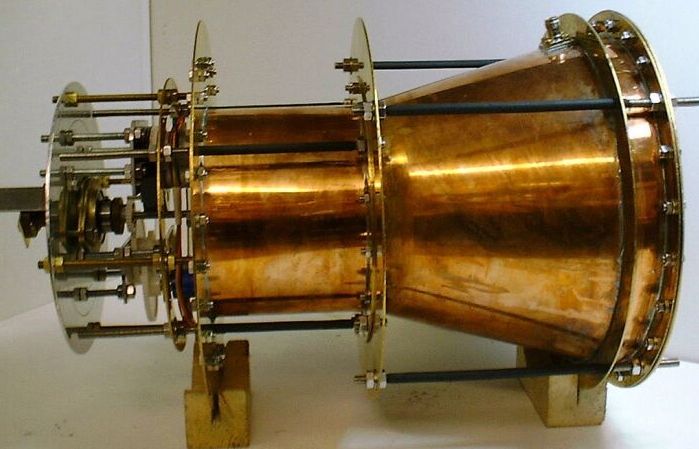
The report, titled “Measurement of Impulsive Thrust from a Closed Radio Frequency Cavity in Vacuum“, was apparently leaked in early November. It’s lead author is predictably Harold White, the Advanced Propulsion Team Lead for the NASA Engineering Directorate and the Principal Investigator for NASA’s Eagleworks lab.

As he and his colleagues (allegedly) report in the paper, they completed an impulsive thrust test on a “tapered RF test article”. This consisted of a forward and reverse thrust phase, a low thrust pendulum, and three thrust tests at power levels of 40, 60 and 80 watts. As they stated in the report:

“It is shown here that a dielectrically loaded tapered RF test article excited in the TM212 mode at 1,937 MHz is capable of consistently generating force at a thrust level of 1.2 ± 0.1 mN/kW with the force directed to the narrow end under vacuum conditions.”

Ionic propulsion is currently the slowest, but fmost fuel-efficient, form of space travel. Credit: NASA/JPL — *Ionic propulsion is currently the slowest, but most fuel-efficient, form of space travel. Credit: NASA/JPL*

To be clear, this level of thrust to power – 1.2. millinewtons per kilowatt – is quite insignificant. In fact, the paper goes on to place these results in context, comparing them to ion thrusters and laser sail proposals:

“The current state of the art thrust to power for a Hall thruster is on the order of 60 mN/kW. This is an order of magnitude higher than the test article evaluated during the course of this vacuum campaign… The 1.2 mN/kW performance parameter is two orders of magnitude higher than other forms of ‘zero propellant’ propulsion such as light sails, laser propulsion and photon rockets having thrust to power levels in the 3.33-6.67 [micronewton]/kW (or 0.0033 – 0.0067 mN/kW) range.”

Currently, ion engines are considered the most fuel-efficient form of propulsion. However, they are notoriously slow compared to conventional, solid-propellant thrusters. To offer some perspective, NASA’s Dawn mission relied on a xenon-ion engine that had a thrust to power generation of 90 millinewtons per kilowatt. Using this technology, it took the probe almost four years to travel from Earth to the asteroid Vesta.

The concept of direct-energy (aka. laser sails), by contrast, requires very little thrust since it involves wafer-sized craft – tiny probes which weight about a gram and carry all their instruments they need in the form of chips. This concept is currently being explored for the sake of making the journey to neighboring planets and star systems within our own lifetimes.

Two good examples are the NASA-funded DEEP-IN interstellar concept that is being developed at UCSB, which attempts to use lasers to power a craft up to 0.25 the speed of light. Meanwhile, Project Starshot (part of Breakthrough Initiatives) is developing a craft which they claim will reach speeds of 20% the speed of light, and thus be able to make the trip to Alpha Centauri in 20 years.

Compared to these proposals, the EM Drive can still boast the fact that it does not require any propellant or an external power source. But based on these test results, the amount of power that would be needed to generate a significant amount of thrust would make it impractical. However, one should keep in mind that this low power test was designed to see if any thrust detected could be attributed to anomalies (none of which were detected).

The report also acknowledges that further testing will be necessary to rule out other possible causes, such as center of gravity (CG) shifts and thermal expansion. And if outside causes can again be ruled out, future tests will no doubt attempt to maximize performance to see just how much thrust the EM Drive is capable of generating.

But of course, this is all assuming that the “leaked” paper is genuine. Until NASA can confirm that these results are indeed real, the EM Drive will be stuck in controversy limbo. And while we’re waiting, check out this descriptive video by astronomer Scott Manley from the Armagh Observatory:

Further Reading: Science Alert

November 10, 2016November 11, 2016 by Matt Williams

Discovery Of A Nearby Super Earth With Only 5 Times Our Mass

Artists impression of a Super-Earth, a class of planet that has many times the mass of Earth, but less than a Uranus or Neptune-sized planet. Credit: NASA/Ames/JPL-Caltech

Red dwarf stars have proven to be a treasure trove for exoplanet hunters in recent years. In addition to multiple exoplanets candidates being detected around stars like TRAPPIST-1, Gliese 581, Gliese 667C, and Kepler 296, there was also the ESO’s recent discovery of a planet orbiting within the habitable zone of our Sun’s closest neighbor – Proxima Centauri.

And it seems the trend is likely to continue, with the latest discovery comes from a team of European scientists. Using data from the ESO’s High Accuracy Radial velocity Planet Searcher (HARPS) and HARPS-N instruments, they detected an exoplanet candidate orbiting around GJ 536 – an M-class red dwarf star located about 32.7 light years (10.03 parsecs) from Earth.

According to their study, “A super-Earth Orbiting the Nearby M-dwarf GJ 536“, this planet is a super-Earth – a class of exoplanet that has between more than one, but less than 15, times the mass of Earth. In this case, the planet boasts a minimum of 5.36 ± 0.69 Earth masses, has an orbital period of 8.7076 ± 0.0025 days, and orbits its sun at a distance of 0.06661 AU.

Artist's impression of a system of exoplanets orbiting a low mass, red dwarf star. Credit: NASA/JPL — *Artist’s impression of a system of exoplanets orbiting a low mass, red dwarf star. Credit: NASA/JPL*

The team was led by Dr. Alejandro Suárez Mascareño of the Instituto de Astrofísica de Canarias (IAC). The discovery of the planet was part of his thesis work, which was conducted under Dr Rafael Rebolo – who is also a member of the IAC, the Spanish National Research Council and a professor at the University of Laguna. And while the planet is not a potentially habitable world, it does present some interesting opportunities for exoplanet research.

As Dr. Mascareño shared with Universe Today via email:

“GJ 536 b is a small super Earth discovered in a very nearby star. It is part of the group of the smallest planets with measured mass. It is not in the habitable zone of its star, but its relatively close orbit and the brightness of its star makes it a promising target for transmission spectroscopy IF we can detect the transit. With a star so bright (V 9.7) it would be possible to obtain good quality spectra during the hypothetical transit to try to detect elements in the atmosphere of the planet. We are already designing a campaign for next year, but I guess we won’t be the only ones.”

The survey that found this planet was part of a joint effort between the IAC (Spain) and the Geneva Observatory (Switzerland). The data came from the HARPS and HARPS-N instruments, which are mounted on the ESO’s 3.6 meter telescope at the La Silla Observstory in Chile and the 3.6 meter telescope at the La Palma Observatory in Spain. This was combined with photometric data from the All Sky Automated Survey (ASAS), which has observatories in Chile and Maui.

The research team relied on radial velocity measurements from the star to discern the presence of the planet, as well as spectroscopic observations of the star that were taken over a 8.6 year period. For all this, they not only detected an exoplanet candidate with 5 times the mass of Earth, but also derived information on the star itself – which showed that it has a rotational period of about 44 days, and magnetic cycle that lasts less than three years.

Artist's depiction of the interior of a low-mass star, such as the one seen in an X-ray image from Chandra in the inset. Credit: NASA/CXC/M.Weiss — *Artist’s depiction of the interior of a low-mass star, such as the one seen in an X-ray image from Chandra in the inset. Credit: NASA/CXC/M.Weiss*

By comparison, our Sun has a rotational period of 25 days and a magnetic cycle of 11 years, which is characterized by changes in the levels of solar radiation it emits, the ejection of solar material and in the appearance of sunspots. In addition, a recent study from the the Harvard Smithsonian Center for Astrophysics (CfA) showed that Proxima Centauri has a stellar magnetic cycle that lasts for 7 years.

This detection is just the latest in a long line of exoplanets being discovered around low-mass, low-luminosity, M-class (red dwarf) stars. And looking ahead, the team hopes to continue surveying GJ 536 to see if there is a planetary system, which could include some Earth-like planets, and maybe even a few gas giants.

“For now we have detected only one planet, but we plan to continue monitoring the star to search for other companions at larger orbital separations,” said Dr. Mascareño. “We estimate there is still room for other low-mass or even Neptune-mass planets at orbits from a hundred of days to a few years.”

The research also included scientists from the Astronomical Observatory at the University of Geneva, the University of Grenoble, The Astrophysical and Planetological Insitute of Grenoble, Institute of Astrophysics and Space Sciences in Portugal, and the University of Porto, Portugal.

Further Reading: arXiv

November 10, 2016February 3, 2017 by David Dickinson

Preview: Comet 45P/Honda–Mrkos–Pajdušáková Brightens in December

Comet 45P/Honda-Mrkos-Pajdušáková From October 1st, 2011 taken with a 10"/3.8 Newtonian and CCD imager. Image credit and copyright: Michael Jäger.

Looking for a good binocular comet? Well, if luck is on our side, we should be getting our first looks at periodic Comet 45P/Honda-Mrkos-Pajdušáková as it tops +10th magnitude in dusk skies over the next few weeks.

The swift path of Comet 45P/Honda-Mrkos-Pajdušáková on the nights of February 9th to February 12th. Image credit: Starry Night.

Comet 45P/Honda-Mrkos-Pajdušáková is expected to reach maximum brightness around late February 2017. Discovered independently by astronomers Minoru Honda, Antonin Mrkos and L’udmila Pajdušáková on December 3^rd, 1948, Comet 45P/Honda-Mrkos-Pajdušáková orbits the Sun once every 5.25 years on a short period orbit. Comet 45P/Honda-Mrkos-Pajdušáková is set to break binocular +10^th magnitude brightness in mid-December 2017, and may reach a maximum brightness of magnitude +7 from January through February 2017.

Slovak astronomer ?udmila Pajdušáková, co-discoverer of 5 comets, including Comet 45P/Honda-Mrkos-Pajdušáková. Image credit: The Skalnaté Pleso Observatory.

Currently and through the end of 2016, the comet sits towards the center of the Milky Way Galaxy in Sagittarius at a faint +15^th magnitude in the evening sky. The comet may break +10^th magnitude and become very briefly visible in the first few weeks of December before getting too close to the Sun to observe in late 2016 and crossing into the morning sky in early 2017.

The path of Comet 45/P from mid-November through December 15th, 2016. Image credit: Starry Night.

Visibility prospects: At its brightest, Comet 45P/Honda-Mrkos-Pajdušáková will be passing through the constellation Hercules during closest approach on February 11^th. The comet then passes through the constellations of Corona Borealis, Boötes, Canes Venatici, Ursa Major into Leo through to the end of February as it recedes. In the second week of February, the comet is visible in the dawn sky 82 degrees west of the Sun at maximum brightness. This apparition favors the northern hemisphere. The comet will reach perihelion on December 29^th, 2016 at 0.53 Astronomical Units (AU) from the Sun, and the comet passes just 0.08 AU (7.4 million miles) from the Earth on February 11^th at 14:44 UT. The comet made a slightly closer pass in 2011, and was a fine binocular object that time around. At its closest, the comet will cross nine degrees of sky from one night to the next. Some notable dates for comet 45P/Honda-Mrkos-Pajdušáková are:

November 23^rd: Venus passes 6′ from the comet.

December 12^th: May break 10^th magnitude.

December 14^th: Passes near M75.

December 15^th: Crosses into the constellation Capricornus.

January 4^th: Passes near the +4^th magnitude star Theta Capricorni

January 10^th: Crosses the ecliptic northward.

January 16^th: Passes into Aquarius.

January 22^nd: Passes near NGC 7009, M72 and M73.

January 25^th: Passes 8 degrees from the Sun and into the dawn sky.

January 28^th: Crosses into Aquila.

February 3^rd: Crosses the celestial equator northward.

February 4^th: Passes 4′ from the star +3.3 magnitude star Delta Aquilae.

February 6^th: Crosses the Galactic equator.

February 7^th: Crosses into Ophiuchus.

February 9^th: Crosses into Hercules.

February 16^th: makes a wide pass near M3.

February 19^th: Drops back below +10^th magnitude.

The path of Comet 45P/Honda-Mrkos-Pajdušáková through the inner solar system. Image credit: NASA/JPL.

This is the final close (less than 0.1 AU) passage of Comet 45P/Honda-Mrkos-Pajdušáková near the Earth for this century.

On July 1^st 1770, Comet D/1770 L1 Lexell passed 0.0151AU from the Earth; a comet in 1491 may have passed closer. Next year’s passage of 45P/Honda-Mrkos-Pajdušáková ranks as the 21^st closest passage of a comet near the Earth.

The light curve of Comet 45/P Honda-Mrkos-Pajdušáková. Credit: Seiichi Yoshida’s *Weekly Information About Bright Comets.*

Why do comets end up with such cumbersome names? Well, comets derive their names from the first three discovers that submit the find within a 24 hour period to the Minor Planet Center’s Central Bereau for Astronomical Telegrams, which, in fact, received its last ‘telegram’ during the discovery of Comet Hale-Bopp around two decades ago. Increasingly, comets are receiving names of all sky surveys such as LINEAR and PanSTARRS from robotic competition against amateur hunters. It does seem like you need an umlaut or the chemical symbol for boron to in your moniker to qualify these days… rare is the ‘Comet Smith.’ But hey, it’s still fun to watch science journalists try and spell the Icelandic volcano Eyjafjallajökull and comet Churyumov-Gerasimenko over and over… Perhaps, we should insist that our first comet discovery is actually spelled Comet Dîckînsðn…

And Comet 45/P is just one of the fine binocular comets on deck for 2017. We’re also expecting Comet 41P/Tuttle-Giacobini-Kresák, 2/P Encke, C/2015 ER61 PanSTARRS Comet C/2015 V2 Johnson to break +10^th magnitude next year… and the next great naked eye ‘Comet of the Century’ could light up the skies at any time.

Goldstone radar pings comet 45/P back in 2011. Image credit: NASA.

Binoculars are the best tool to observe bright comets, as they allow you to simply sweep the star field and admire the full beauty of a comet, coma, tail(s) and all. Keep in mind, a comet will often appear visually fainter than its quoted brightness… this is because, like nebulae, that intrinsic magnitude is ‘smeared out’ over an extended area. To my eye, a binocular comet often looks like a fuzzy, unresolved globular cluster that stubbornly refuses to snap into focus.

Don’t miss your first looks at Comet 45/P 45P/Honda-Mrkos-Pajdušáková, as it spans 2016 into 2017.

November 9, 2016November 11, 2016 by Matt Williams

Where Will President-Elect Trump Take American Space Endeavours?

Given the fiscal policies of his party, and his own stances on Climate Change, there is concern about how a Trump administration will affect NASA. Credit: Wikipedia Commons/Gage Skidmore

With the 2016 election now finished and Donald Trump confirmed as the president-elect of the United States, there are naturally some concerns about what this could means for the future of NASA. Given the administration’s commitment to Earth science, and its plans for crewed missions to near-Earth Orbit and Mars, there is understandably some worry that the budget environment might be changing soon.

At this juncture, it is not quite clear how a Trump presidency will affect NASA’s mandate for space exploration and scientific research. But between statements made by the president-elect in the past, and his stances on issues like climate change, it seems clear that funding for certain types of research could be threatened. But there is also reason to believe that larger exploration programs might be unaffected.

Back in September, the Senate Committee on Commerce, Science, and Transportation passed the NASA Transition Authorization Act of 2016. This bill granted $19.5 billion in funding for NASA for fiscal year 2017, thus ensuring that NASA’s proposed activities would not be affected by the transition in power. Central to this bill was the continued funding of operations that NASA considered to be central to its “Journey to Mars“.

Looking forward, it is unclear how the new administration will affect NASA's plans for space exploration. Credit: NASA/AESP — Looking forward, it is unclear how the new administration will affect NASA’s plans for space exploration. Credit: NASA/AESP

Beyond FY 2017, though, the picture is unclear. When it comes to things like NASA’s Earth Science program, the administration of a president that denies the existence of Climate Change is expected to mean budget cuts. For instance, back in May, Trump laid out his vision for an energy policy. Central to this was a focus on oil, natural gas and coal, the cancellation of the Paris Agreement, and the cessations of all payments to the UN Green Climate Fund.

This could signal a possible reverse of policies initiated by the Obama administration, which increased funding for Earth science research by about 50 percent. And as NASA indicated in a report issued on Nov. 2nd by the Office of the Inspect General – titled “NASA’s Earth Science Mission Portfolio” – this has resulted in some very favorable developments.

Foremost among these has been the increased in the number of products delivered to users by NASA, going from 8.14 million in 2000 to 1.42 billion in 2015. In other words, usage of NASA resources has increased by a factor of 175, and in the space of just 15 years (much of that in the last 8). Another major benefit has been the chance for collaboration and lucrative partnerships. From the report:

“Government agencies, scientists, private entities, and other stakeholders rely on NASA to process raw information received from Earth observation systems into useable data. Moreover, NASA’s Earth observation data is routinely used by government agencies, policy makers, and researchers to expand understanding of the Earth system and to enhance economic competitiveness, protect life and property, and develop policies to help protect the planet. Finally, NASA is working to address suggestions that it use commercially provided data to augment its Earth observation data. However, NASA must reconcile its policy that promotes open sharing of data at minimal cost to users with a commercial business model under which fees may create a barrier to use.”

Much of NASA's research into Climate Change takes place through the Earth Sciences Directorate. Credit: NASA — *Much of NASA’s research into Climate Change takes place through the Earth Science division of the Mission Directorate. Credit: NASA*

Unfortunately, it has been this same increase in funding that prompted Congressional Republicans, in the name of fiscal responsibility, to demand changes and new standards. These sentiments were voiced back in March of 2015 during NASA’s budget request for 2016. As Senator Ted Cruz – currently one of the Trump campaign’s backers – said at the time:

“We’ve seen a disproportionate increase in the amount of federal funds going to the earth sciences program at the expense of funding for exploration and space operations, planetary sciences, heliophysics, and astrophysics, which I believe are all rooted in exploration and should be central to NASA’s core mission. We need to get back to the hard sciences, to manned space exploration, and to the innovation that has been integral to NASA.

While Trump himself has little to say about space during his long campaign, his team did manage to recruit Robert Walker – a former Republican congressman from Pennsylvania – this past October to draft a policy for them. In an op-ed to SpaceNews in late October, he echoed Cruz’s sentiments about cutting back on Earth sciences to focus on space exploration:

“NASA should be focused primarily on deep space activities rather than Earth-centric work that is better handled by other agencies. Human exploration of our entire solar system by the end of this century should be NASA’s focus and goal. Developing the technologies to meet that goal would severely challenge our present knowledge base, but that should be a reason for exploration and science.”

“It makes little sense for numerous launch vehicles to be developed at taxpayer cost, all with essentially the same technology and payload capacity. Coordinated policy would end such duplication of effort and quickly determine where there are private sector solutions that do not necessarily require government investment.“

NASA's Journey to Mars. NASA is developing the capabilities needed to send humans to an asteroid by 2025 and Mars in the 2030s. Credit: NASA/JPL — *NASA is developing the capabilities needed to send humans to an asteroid by 2025 and Mars in the 2030s. Credit: NASA/JPL*

Next, there is the issue of NASA’s long-term goals, which (as noted) seem more secure for the time being. In May of 2016, Trump was issued the Aerospace America Questionnaire – a series of ten questions issued by NASA to determine the stances of the candidates on space exploration. On the subject of a crewed mission to Mars in the future, Trump’s campaign indicated that things would depend upon the state of the country’s economy:

“A lot of what my administration would recommend depends on our economic state. If we are growing with all of our people employed and our military readiness back to acceptable levels, then we can take a look at the timeline for sending more people into space.“

However, they also professed an admiration for NASA and a commitment to its overall goal:

“NASA has been one of the most important agencies in the United States government for most of my lifetime. It should remain so. NASA should focus on stretching the envelope of space exploration for we have so much to discover and to date we have only scratched the surface.”

From all of this, a general picture of what NASA’s budget environment will look like in the near future begins to emerge. In all likelihood, the Earth Science division (and other parts of NASA) are likely to find their budgets being scrutinized based on newly-developed criteria. Essentially, unless it benefits space exploration and research beyond Earth, it’s not likely to see continued funding.

*NASA Administrator Charles Bolden. Credit: NASA*

But regardless of the results of the election, it appears at this juncture that NASA is looking forward with cautious optimism. Addressing the future, NASA Administrator Charles Bolden issued an internal memo on Wednesday, Nov. 9th. Titled “Reaching for New Heights in 2017 and Beyond“, Bolden expressed positive thoughts about the transition of power and what it would mean:

“In times when there has been much news about all the things that divide our nation, there has been noticeable bipartisan support for this work, our work – support that not only reaches across the aisle, but across the public, private, academic and non-profit sectors.

“For this reason, I think we can all be confident that the new Trump Administration and future administrations after that will continue the visionary course on which President Barack Obama has set us, a course that all of you have made possible.”

For NASA’s sake, I hope Bolden’s words prove to be prophetic. For no matter who holds of the office of the President of the United States, the American people – and indeed, all the world’s people – depend upon the continued efforts of NASA. As the leader in space exploration, their presence is essential to humanity’s return to space!

Further Reading: Planetary Society

November 9, 2016November 9, 2016 by David Dickinson

November’s Supermoon 2016 – Closest of a Lifetime?

The 2015 Supermoon. Image credit and copyright: Wils 888.

What’s that, rising in the sky?

By now, you’ve heard the news. We’ll spare you the “it’s a bird, it’s a plane…” routine to usher in the Supermoon 2016. This month’s Full Moon is not only the closest for the year, but the nearest Full Moon for a 80 year plus span.

Like Blue and Black Moons, a Supermoon is more of a cultural phenomenon than a true astronomical event. The Moon’s orbit is elliptical, taking it from 362,600 to 405,400 km from the Earth in the course of its 27.55 day anomalistic orbit from one perigee to the next. For the purposes of this week’s discussion, we consider a Supermoon as when the Full Moon occurs within 24 hours of perigee, and a Minimoon as when the Full Moon occurs within 24 hours of apogee. From the Earth, the Moon varies in apparent size from 29.3” to 34.1” across. This month, the Moon reaches perigee on November 14^th at 356,511 kilometers distant, 2 hours and 22 minutes before Full.

A perigee 'Supermoon' versus an apogee 'Minimoon'. Image credit and copyright: Raven Yu. — A perigee ‘Supermoon’ versus an apogee ‘Minimoon’. Image credit and copyright: Raven Yu.

This is the closest perigee Moon for 2016, beating out the April 7^th, 2016 perigee Moon by just 652 kilometers. Perigee can vary over a span of 2,800 kilometers. In the 21^st century, the farthest lunar perigee (think the ‘most distant near point’) occurs on January 3^rd, 2100 at 370,356 kilometers distant, while the closest perigee of the century (356,425 kilometers) occurs on December 6^th , 2052.

When the Moon reaches Full on November 14^th at 13:51 UT, it’s just 356,520 kilometers distant, (that is , as measured from the Earth’s center) the closest Full Moon since January 26^th, 1948 (356,490 km) and until November 25^th , 2034 (356,446 km) losing out to either dates by just 21 kilometers.

Why does perigee vary? Well, as the Moon orbits the Earth, the Sun tugs our large natural satellite’s orbit around as well, in an 8.85 year cycle known as the precession of the line of apsides. Earth’s orbit is elliptical as well, and the tugging of the Sun (and to a much lesser degree, the other planets in the solar system) alters the perigee and apogee points slightly based on where the Earth-Moon pair fall in their swing about a common barycenter.

The November Full Moon is also known as the Full Beaver Moon by the Algonquin Native Americans, a good time to ensure a supply of winter furs before the swamps froze over. A good sign that even in 2016, ‘Winter is Coming.’

Does the Moon look any larger to you than usual as it rises to the east opposite to the setting Sun on Monday night? When the Moon reaches Full, it passes the zenith as seen from the central Indian Ocean region just south of Sri Lanka, 354,416 km distant. Of course, as the Moon rises, it’s actually one full Earth radii more distant than when straight overhead at the zenith.

A side-by-side 'Super' vs 'Minimoon.' Image credit and copyright: Marco Langbroek. — A side-by-side ‘Super’ vs ‘Minimoon.’ Image credit and copyright: Marco Langbroek.

Would you notice any difference in the size of the November Full Moon, if you didn’t know better? The 4′ odd difference between an apogee and perigee Full Moon is certainly discernible in side-by-side images… but it’s interesting to note that early cultures did not uncover the elliptical nature of the Moon’s motion, though it certainly would have been possible. Crystalline spheres ruled the day, a sort of perfection that was just tough to break in the minds of many.

Be sure to enjoy the rising Full Moon on Monday night, the largest for many years to come.

November 8, 2016August 25, 2021 by Matt Williams

What are Active Galactic Nuclei?

An artist's impression of the accretion disc around the supermassive black hole that powers an active galaxy. Astronomers want to know if the energy radiated from a black hole is caused by jets of material shooting away from the hole, or by the accretion disk of swirling material near the hole. Credit: NASA/Dana Berry, SkyWorks Digital

In the 1970s, astronomers became aware of a compact radio source at the center of the Milky Way Galaxy – which they named Sagittarius A. After many decades of observation and mounting evidence, it was theorized that the source of these radio emissions was in fact a supermassive black hole (SMBH). Since that time, astronomers have come to theorize that SMBHs at the heart of every large galaxy in the Universe.

Most of the time, these black holes are quiet and invisible, thus being impossible to observe directly. But during the times when material is falling into their massive maws, they blaze with radiation, putting out more light than the rest of the galaxy combined. These bright centers are what is known as Active Galactic Nuclei, and are the strongest proof for the existence of SMBHs.

Description:

It should be noted that the enormous bursts in luminosity observed from Active Galactic Nuclei (AGNs) are not coming from the supermassive black holes themselves. For some time, scientists have understood that nothing, not even light, can escape the Event Horizon of a black hole.

Instead, the massive burst of radiations – which includes emissions in the radio, microwave, infrared, optical, ultra-violet (UV), X-ray and gamma ray wavebands – are coming from cold matter (gas and dust) that surround the black holes. These form accretion disks that orbit the supermassive black holes, and gradually feeding them matter.

The incredible force of gravity in this region compresses the disk’s material until it reaches millions of degrees kelvin. This generates bright radiation, producing electromagnetic energy that peaks in the optical-UV waveband. A corona of hot material forms above the accretion disc as well, and can scatter photons up to X-ray energies.

A large fraction of the AGN’s radiation may be obscured by interstellar gas and dust close to the accretion disc, but this will likely be re-radiated at the infrared waveband. As such, most (if not all) of the electromagnetic spectrum is produced through the interaction of cold matter with SMBHs.

The interaction between the supermassive black hole’s rotating magnetic field and the accretion disk also creates powerful magnetic jets that fire material above and below the black hole at relativistic speeds (i.e. a significant fraction of the speed of light). These jets can extend for hundreds of thousands of light-years, and are a second potential source of observed radiation.

Types of AGN:

Typically, scientists divide AGN into two categories, which are referred to as “radio-quiet” and “radio-loud” nuclei. The radio-loud category corresponds to AGNs that have radio emissions produced by both the accretion disk and the jets. Radio-quiet AGNs are simpler, in that any jet or jet-related emission are negligible.

Carl Seyfert discovered the first class of AGN in 1943, which is why they now bear his name. “Seyfert galaxies” are a type of radio-quiet AGN that are known for their emission lines, and are subdivided into two categories based on them. Type 1 Seyfert galaxies have both narrow and broadened optical emissions lines, which imply the existence of clouds of high density gas, as well as gas velocities of between 1000 – 5000 km/s near the nucleus.

Type 2 Seyferts, in contrast, have narrow emissions lines only. These narrow lines are caused by low density gas clouds that are at greater distances from the nucleus, and gas velocities of about 500 to 1000 km/s. As well as Seyferts, other sub classes of radio-quiet galaxies include radio-quiet quasars and LINERs.

Low Ionisation Nuclear Emission-line Region galaxies (LINERs) are very similar to Seyfert 2 galaxies, except for their low ionization lines (as the name suggests), which are quite strong. They are the lowest-luminosity AGN in existence, and it is often wondered if they are in fact powered by accretion on to a supermassive black hole.

Artist's representation of an active galactic nucleus (AGN) at the center of a galaxy. Credit: NASA/CXC/M.Weiss — Artist’s representation of an active galactic nucleus (AGN) at the center of a galaxy. Credit: NASA/CXC/M.Weiss

Radio-loud galaxies can also be subdivded into categories like radio galaxies, quasars, and blazars. As the name suggests, radio galaxies are elliptical galaxies that are strong emitters of radiowaves. Quasars are the most luminous type of AGN, which have spectra similar to Seyferts.

However, they are different in that their stellar absorption features are weak or absent (meaning they are likely less dense in terms of gas) and the narrow emission lines are weaker than the broad lines seen in Seyferts. Blazars are a highly variable class of AGN that are radio sources, but do not display emission lines in their spectra.

Detection:

Historically speaking, a number of features have been observed within the centers of galaxies that have allowed for them to be identified as AGNs. For instance, whenever the accretion disk can be seen directly, nuclear-optical emissions can be seen. Whenever the accretion disk is obscured by gas and dust close to the nucleus, an AGN can be detected by its infra-red emissions.

Then there are the broad and narrow optical emission lines that are associated with different types of AGN. In the former case, they are produced whenever cold material is close to the black hole, and are the result of the emitting material revolving around the black hole with high speeds (causing a range of Doppler shifts of the emitted photons). In the former case, more distant cold material is the culprit, resulting in narrower emission lines.

Image taken by the Hubble Space Telescope of a 5000-light-year-long jet ejected from the active galaxy M87. The blue synchrotron radiation contrasts with the yellow starlight from the host galaxy. Credit: NASA/The Hubble Heritage Team (STScI/AURA) — *Image taken by the Hubble Space Telescope of a 5000-light-year-long jet ejected from the active galaxy M87. Credit: NASA/The Hubble Heritage Team (STScI/AURA)*

Next up, there are radio continuum and x-ray continuum emissions. Whereas radio emissions are always the result of the jet, x-ray emissions can arise from either the jet or the hot corona, where electromagnetic radiation is scattered. Last, there are x-ray line emissions, which occur when x-ray emissions illuminate the cold heavy material that lies between it and the nucleus.

These signs, alone or in combination, have led astronomers to make numerous detections at the center of galaxies, as well as to discern the different types of active nuclei out there.

The Milky Way Galaxy:

In the case of the Milky Way, ongoing observation has revealed that the amount of material accreted onto Sagitarrius A is consistent with an inactive galactic nucleus. It has been theorized that it had an active nucleus in the past, but has since transitioned into a radio-quiet phase. However, it has also been theorized that it might become active again in a few million (or billion) years.

When the Andromeda Galaxy merges with our own in a few billion years, the supermassive black hole that is at its center will merge with our own, producing a much more massive and powerful one. At this point, the nucleus of the resulting galaxy – the Milkdromeda (Andrilky) Galaxy, perhaps? – will certainly have enough material for it to be active.

The discovery of active galactic nuclei has allowed astronomers to group together several different classes of galaxies. It’s also allowed astronomers to understand how a galaxy’s size can be discerned by the behavior at its core. And last, it has also helped astronomers to understand which galaxies have undergone mergers in the past, and what could be coming for our own someday.

We have written many articles about galaxies for Universe Today. Here’s What Fuels the Engine of a Supermassive Black Hole?, Could the Milky Way Become a Black Hole?, What is a Supermassive Black Hole?, Turning on a Supermassive Black Hole, What Happens when Supermassive Black Holes Collide?.

For more information, check out Hubblesite’s News Releases on Galaxies, and here’s NASA’s Science Page on Galaxies.

Astronomy Cast also has episodes about galactic nuclei and supermassive black holes. Here’s Episode 97: Galaxies and Episode 213: Supermassive Black Holes.

Source:

November 8, 2016November 8, 2016 by Matt Williams

What are Magellanic Clouds?

The night sky above the Danish 1.54-metre telescope at ESO's La Silla Observatory. The Magellanic Clouds are visible to the right of the central bar of the Milky Way. Credit: ESO/Z. Bardon

Since ancient times, human beings have been staring at the night sky and been amazed by the celestial objects looking back at them. Whereas these objects were once thought to be divine in nature, and later mistaken for comets or other astrological phenomena, ongoing observation and improvements in instrumentation have led to these objects being identified for what they are.

For example, there are the Small and Large Magellanic Clouds, two large clouds of stars and gas that can be seen with the naked eye in the southern hemisphere. Located at a distance of 200,000 and 160,000 light years from the Milky Way Galaxy (respectively), the true nature of these objects has only been understand for about a century. And yet, these objects still have some mysteries that have yet to be solved.

Characteristics:

The Large Magellanic Cloud (LMC) and the neighboring the Small Magellanic Cloud (SMC) are starry regions that orbit our galaxy, and look conspicuously like detached pieces of the Milky Way. Though they are separated by 21 degrees in the night sky – about 42 times the width of the full moon – their true distance is about 75,000 light-years from each other.

An ultraviolet view of the Large Magellanic Cloud from Swift's Ultraviolet/Optical Telescope. Almost 1 million ultraviolet sources are visible in the image, which took 5.4 days of cumulative exposure to do. The wavelengths of UV shown in this picture are mostly blocked on Earth's surface. Credit: NASA/Swift/S. Immler (Goddard) and M. Siegel (Penn State) — *Ultraviolet view of the Large Magellanic Cloud from Swift’s Ultraviolet/Optical Telescope. Credit: NASA/Swift/S. Immler (Goddard) and M. Siegel (Penn State)*

The Large Magellanic Cloud is located about 160,000 light-years from the Milky Way, in the constellation Dorado. This makes it the 3rd closest galaxy to us, behind the Sagittarius Dwarf and Canis Major Dwarf galaxies. Meanwhile, the Small Magellanic Cloud is located in the constellation of Tucana, about 200,000 light-years away.

The LMC is roughly twice the diameter of the SMC, measuring some 14,000 light-years across vs. 7,000 light years (compared to 100,000 light years for the Milky Way). This makes it the 4th largest galaxy in our Local Group of galaxies, after the Milky Way, Andromeda and the Triangulum Galaxy. The LMC is about 10 billion times as massive as our Sun (about a tenth the mass of the Milky Way), while the SMC is equivalent to about 7 billion Solar Masses.

In terms of structure, astronomers have classified the LMC as an irregular type galaxy, but it does have a very prominent bar in its center. Ergo, it’s possible that it was a barred spiral before its gravitational interactions with the Milky Way. The SMC also contains a central bar structure and it is speculated that it too was once a barred spiral galaxy that was disrupted by the Milky Way to become somewhat irregular.

Aside from their different structure and lower mass, they differ from our galaxy in two major ways. First, they are gas-rich – meaning that a higher fraction of their mass is hydrogen and helium – and they have poor metallicity, (meaning their stars are less metal-rich than the Milky Way’s). Both possess nebulae and young stellar populations, but are made up of stars that range from very young to the very old.

The Small Magellanic Cloud as seen by Swift's Ultraviolet/Optical Telescope. This composite of 656 separate pictures has a cumulative exposure time of 1.8 days. Credit: NASA/Swift/S. Immler (Goddard) and M. Siegel (Penn State) — The Small Magellanic Cloud as seen by Swift’s Ultraviolet/Optical Telescope. This composite of 656 separate pictures has a cumulative exposure time of 1.8 days. Credit: NASA/Swift/S. Immler (Goddard) and M. Siegel (Penn State)

In fact, this abundance in gas is what ensures that the Magellanic Clouds are able to create new stars, with some being only a few hundred million years in age. This is especially true of the LMC, which produces new stars in large quantities. A good example of this is it’s glowing-red Tarantula Nebula, a gigantic star-forming region that lies 160,000 light-years from Earth.

Astronomers estimate that the Magellanic Clouds were formed approximately 13 billion years ago, around the same time as the Milky Way Galaxy. It has also been believed for some time that the Magellanic Clouds have been orbiting the Milky Way at close to their current distances. However, observational and theoretical evidence suggests that the clouds have been greatly distorted by tidal interactions with the Milky Way as they travel close to it.

This indicates that they are not likely to have frequently got as close to the Milky Way as they are now. For instance, measurements conducted with the Hubble Space Telescope in 2006 suggested that the Magellanic Clouds may be moving too fast to be long terms companions of the Milky Way. In fact, their eccentric orbits around the Milky Way would seem to indicate that they came close to our galaxy only once since the universe began.

Small and Large Magellanic Clouds over Paranal Observatory Credit: ESO/J. Colosimo — *The Small and Large Magellanic Clouds visible over the Paranal Observatory in Chile. Credit: ESO/J. Colosimo*

This was followed in 2010 by a study that indicated that the Magellanic Clouds may be passing clouds that were likely expelled from the Andromeda Galaxy in the past. The interactions between the Magellanic Clouds and the Milky Way is evidenced by their structure and the streams of neutral hydrogen that connects them. Their gravity has affected the Milky Way as well, distorting the outer parts of the galactic disk.

History of Observation:

In the southern hemisphere, the Magellanic clouds were a part of the lore and mythology of the native inhabitants, including the Australian Aborigines, the Maori of New Zealand, and the Polynesian people of the South Pacific. For the latter, they served as important navigational markers, while the Maori used them as predictors of the winds.

While the study Magellanic Clouds dates back to the 1st millennium BCE, the earliest surviving record comes from the 10th century Persian astronomer Al Sufi. In his 964 treatise, Book of Fixed Stars, he called the LMC al-Bakr (“the Sheep”) “of the southern Arabs”. He also noted that the Cloud is not visible from northern Arabia or Baghdad, but could be seen at the southernmost tip of Arabian Peninsula.

By the late 15th century, Europeans are believed to have become acquainted with the Magellanic Clouds thanks to exploration and trade missions that took them south of the equator. For instance, Portuguese and Dutch sailors came to know them as the Cape Clouds, since they could only be viewed when sailing around Cape Horn (South America) and the Cape of Good Hope (South Africa).

Panoramic Large and Small Magellanic Clouds as seen from ESO's VLT observation site. The galaxies are on the left side of the image. Credit: ESO/Y. Beletsky — *Panoramic view of the Large and Small Magellanic Clouds above the ESO’s VLT observation site in Chile. Credit: ESO/Y. Beletsky*

During the circumnavigation of the Earth by Ferdinand Magellan (1519–22), the Magellanic Clouds were described by Venetian Antonio Pigafetta (Magellan’s chronicler) as dim clusters of stars. In 1603, German celestial cartographer Johann Bayer published his celestial atlas Uranometria, where he named the smaller cloud “Nebecula Minor” (Latin for “Little Cloud”).

Between 1834 and 1838, English astronomer John Herschel conducted surveys of the southern skies from the Royal Observatory at the Cape of Good Hope. While observing the SMC, he described it as a cloudy mass of light with an oval shape and a bright center, and catalogued a concentration of 37 nebulae and clusters within it.

In 1891, the Harvard College Observatory opened an observing station in southern Peru. From 1893-1906, astronomers used the observatory’s 61 cm (24 inch) telescope to survey and photograph the LMC and SMC. One such astronomers was Henriette Swan Leavitt, who used the observatory to discover Cephied Variable stars in the SMC.

Her findings were published in 1908 a study titled “1777 variables in the Magellanic Clouds“, in which she showed the relationship between these star’s variability period and luminosity – which became a very reliable means of determining distance. This allowed the SMCs distance to be determined, and became the standard method of measuring the distance to other galaxies in the coming decades.

Hubble image of variable star RS Puppis (NASA, ESA, and the Hubble Heritage Team) — *Hubble image of variable star RS Puppis, a Cepheid Variable located in the Milky Way Galaxy. Credit: NASA/ESA/Hubble Heritage Team*

As noted already, in 2006, measurements made suing the Hubble Space Telescope were announced that suggested the Large and Small Magellanic Clouds may be moving too fast to be orbiting the Milky Way. This has given rise to the theory that they originated in another galaxy, most likely Andromeda, and were kicked out during a galactic merger.

Given their composition, these clouds – especially the LMC – will continue making new stars for some time to come. And eventually, millions of years from now, these clouds may merge with our own Milky Way Galaxy. Or, they could keep orbiting us, passing close enough to suck up hydrogen and keep their star-forming process going.

But in a few billion years, when the Andromeda Galaxy collides with our own, they may find themselves having no choice but to merge with the giant galaxy that results. One might say Andromeda regrets spitting them out, and is coming to collect them!

We have written many articles about the Magellanic Clouds for Universe Today. Here’s What is the Small Magellanic Cloud?, What is the Large Magellanic Cloud?, Stolen: Magellanic Clouds – Return to Andromeda, The Magellanic Clouds are Here for the First Time.

If you’d like more info on galaxies, check out Hubblesite’s News Releases on Galaxies, and here’s NASA’s Science Page on Galaxies.

We have also recorded an episode of Astronomy Cast about galaxies – Episode 97: Galaxies.

Sources:

November 8, 2016November 8, 2016 by Bob King

What I Learned Writing ‘Night Sky with the Naked Eye’

The author enjoys a pretty display of the northern lights on October 23 under a starry sky. His new book, "Night Sky with the Naked Eye," explores all the amazing things you can see in the sky without special equipment including satellites, planets, meteor showers and of course, the aurora. — The author enjoys a pretty display of the northern lights on October 23, 2016 under a starry sky. His new book, “Night Sky with the Naked Eye,” explores all the amazing things you can see in the sky without special equipment including satellites, planets, meteor showers and of course, the aurora.

My book Night Sky with the Naked Eye publishes today. It would have never seen the light of day much less ever been conceived were it not for Fraser Cain, publisher of Universe Today, and Nancy Atkinson, an editor and writer for the same. Several years ago, Nancy invited me to write for UT. I hopped at the chance. Before her contact, I’d been writing a daily blog on astronomy called Astro Bob (and still do).

Fast forward to last summer when I got an email from Nancy saying Page Street Publishing had contacted her about writing a book about space missions. The publisher also wanted a book about night sky observing without fancy equipment for which she recommended me. Me? I felt like the luckiest guy on the planet!

Book writing proceeds in many stages. First, the table of contents had to be prepared and approved. Then followed a sample chapter. The publisher chose the one on artificial satellites, which I wrote in about a week. The tone was right, but he asked for changes in the organization, which I dutifully made. By November, a contract followed and the project was underway with a first draft due to my editor in about 10 weeks.

Cover of my book that publishes today. Credit: Bob King

Writing is hard work. But it’s a special place all writers come back to again and again. We can’t help but keep trying to find just the right words to capture a concept or emotion. And when we do, a quiet pleasure flows down the spine like warmth creeping into cold fingers splayed in front of a fire. Not that these moments always come easily. Writer Colson Whitehead describes the experience of writing as “crawling through glass.” I would soon become well-acquainted with that feeling, too.

Nancy wrote her book Incredible Stories from Space: A Behind-the-Scenes Look at the Missions Changing Our View of the Cosmos at nearly the same time. We were grateful for each other’s support, and it was a kick to follow her progress as well as bounce ideas around. With a tight deadline in front of me, I set to work immediately, taking more than two weeks of vacation from my regular job to make sure the draft was done on time. No way was I going to compromise an opportunity of a lifetime.

Maybe you’ve thought of writing a book, starting a blog or hope one day to write for Universe Today or another online astronomy site. There’s plenty of good advice for writers out there. I’ll share what worked for me.

#1: Put your butt in the chair and keep it in the chair. My wife reminded me of this often, adding that the book wasn’t going to write itself. Temptations are everywhere. Answering the phone, making another cup of tea, staring out the window and my favorite, shoveling the driveway. I had the cleanest driveway in the neighborhood. Even an inch of new snow was enough to grab the shovel and happily scrape down to the gravel. So yes, I did occasionally get out of the chair, but many times it did me good, freeing up the brain to see more clearly into a topic. Or dream up a fitting photo or illustration.

Creativity comes at odd little moments. It can flow while tapping away in front of a glowing screen or sneak into consciousness when you’re bending down to feed the dog. So a mix of activities seemed the best but with extra emphasis on staying put. I rarely hiked last winter and kept my walks in the neighborhood brief. Instead of observing at night, I wrote or gathered photos. By January, I joked to my friends that I’d voluntarily put myself under house arrest.

#2: Spill your guts, worry about the details later. It’s incredibly tempting when writing to continuously edit one’s work, going back over every sentence to make each “perfect”. This is a muse-killer. Though difficult to stick to, once you let your thoughts flow onto paper without worrying about spelling, clauses and the whole lot of burdensome rules, you’ll become a wild horse running free on the prairie. Let it out, let it out and worry about the commas later. I don’t play a musical instrument, but free-flow writing — just getting the ideas out — must feel something like riffing on a jazz melody.

#3: When stuck, move on to another topic, take a walk, listen to music. Struggling to describe an important concept or connecting your thoughts in a way that flows on the page can drive you nuts, even bring you to tears. Sure, you can keep beating on the idea like a madman hammering on a bent nail, but why why torture yourself? A little distraction can be good. Move on to another part of the story or a different chapter or get up and take a short walk. Defocusing allows the ideas you’re having a tug-of-war with to come of their own accord.

To keep track of ideas, topics and the photos I'd need for the book, I kept a notebook. Credit: Bob King — To keep track of ideas, topics and the photos I’d need for the book, I kept a notebook filled to the gills with lists. Checkmarks indicate tasks accomplished. Credit: Bob King

As the February 1 deadline approached, time took on a physical dimension under the intense pressure to get everything done. I cut time into little blocks that when added up would get me to the finish line on the first draft. I made it just in time, shipped off my copy via e-mail, got in the car to go to work and turn up the music really LOUD. For a fews days I was on top of the world. Invincible.

My editor, Elizabeth, contacted me later with positive comments and then returned the manuscript with “developmental edits” or questions about descriptions and organization. We pitched the ever-refined draft back and forth over the next few months. Each time I read through the ten chapters and made both suggested changes and other refinements. I also added photos during this stage and worked via e-mail with the layout staff to place the best images and graphics at the best places in the text. I shot more images and requested photos from talented astrophotographers, prepared the acknowledgments and sought our recommendations from respected scientists and writers.

This diagram from the book uses the human face to illustrate how changing lighting angles causes the phases of the moon. Credit: Bob King

The editors at Page Street were quite generous with photo usage, a joy for me because that’s what I do for a living. I’ve been a photographer and photo editor at the Duluth News Tribune in Duluth, Minn. for many years. My favorite subjects are people, but I slip in an aurora or eclipse now and again. And that’s the irony. I never saw myself as a writer.

Like many, I started by keeping a journal of my observations through the telescope and reflections about the night sky. The Astro Bob blog took that a step further and writing for Universe Today and Sky & Telescope let me find my voice. So I maybe I have a voice, and I like to think I can be a helpful guide at your side, but writer? That still seems too lofty a term to describe what I do. But here we are.

After several edits including the final one, when I was sent a thick stack of low-res black and white pages of the book to mark up and return, I rested briefly before beginning the final phase: publicity. This is the weird part, where you tell everyone what a nice book you’ve written and how it would make a great Christmas gift for that budding astronomer in the family. When I held the first copy in my hands I couldn’t believe that all those hours of work at the computer became a physical object, a beautiful one even.

This map from the book shows Saturn's location around the time of opposition through 2021. — This map from the book shows Saturn’s location around the time of opposition through 2021. Credit: Bob King, Source: Stellarium

I’m biased of course, but I think both beginning and amateur astronomers will find the book useful. It includes lots of suggested activities – set off in separate boxes – to encourage you to get out under the stars. I make regular mention of the Web and phone apps as ways to become more familiar with the constellations, learn of newly-discovered bright comets and even find a dark sky.

Besides the easy naked eye topics like how to find the brightest constellations or see the best meteor showers of the year, the book offers visual challenges. Have you ever seen craters on the Moon without optical aid or the midnight glow of the gegenschein? You’ll find out how in my book. As a photographer, I’ve included tips on how to focus a digital camera and use it to photograph the aurora or a space station pass.

I’d be willing to bet that most books aren’t as complete as their authors would hope. I had to cut precious photos, graphics, 3 years of a sky calendar and other bits and pieces from mine. Ouch! To this day, I’m still thinking of ways to improve it with a fresh photo, new diagram or change of wording. Now it’s your turn to be the judge.

The zodiacal light punctuated by the planet Jupiter reflects off Lake Superior near Duluth, Minn. this morning (Nov. 8). The book describes nighttime lights such as the zodiacal, gegenschein, airglow and lunar halo and corona phenomena. Credit: Bob King — The zodiacal light punctuated by the planet Jupiter towers over northern Wisconsin along Lake Superior near Duluth, Minn. this morning (Nov. 8). The book describes nighttime lights such as the zodiacal, gegenschein, airglow in addition to lunar halo and corona phenomena. Credit: Bob King

Throughout, Nancy and I rooted for one another and shared our ups and downs. Incredible Stories was to publish within a week of Night Sky, but a type corruption error discovered in several chapters put the book on hold. Her new publication date is December 20, and I encourage you to pre-order a copy, so it arrives in time for Christmas. Order a copy of my book also, and I promise the two of us will keep you company on those long winter nights ahead.

Can I share one final tip? Once you’ve found your passion, say ‘yes’ to every opportunity that furthers it. You’ll be amazed at the places that one word will take you to.

*** To order a copy of Night Sky with the Naked Eye just click an icon to go to the site of your choice — Amazon, Barnes & Noble or Indiebound. It’s currently available at the first two outlets for a very nice discount. It should also be at your local B&N bookstore. And don’t forget to vote today!

November 7, 2016November 21, 2016 by Tammy Plotner

Messier 26 – The NGC 6694 Open Star Cluster

Messier 26 and Delta Scuti. Credit: WIkisky

Welcome back to Messier Monday! In our ongoing tribute to the great Tammy Plotner, we take a look at Messier 26 open star cluster. Enjoy!

Back in the 18th century, famed French astronomer Charles Messier noted the presence of several “nebulous objects” in the night sky. Having originally mistaken them for comets, he began compiling a list of these objects so that others wouldn’t make the same mistake. Consisting of 100 objects, the Messier Catalog would come to be viewed by posterity as a major milestone in the study of Deep Space Objects.

One of these objects is Messier 26, an open star cluster located about 5,000 light years from the Earth in the direction of the Scutum Constellation. While somewhat faint compared to other objects that share its section of the sky, this star field remains a source of mystery to astronomers, thanks to what appears to be a low-density star field at its nucleus.

Description:

When this cloud of stars formed some 89 million years ago, it was probably far more compact than today’s size of a 22 light year span. At a happy distance of about 5,000 light years from our solar system, we can’t quite see into the nucleus to determine just how dense it may actually be because of an obscuring cloud of interstellar matter.

The Open Star Cluster, Messier 26. Credit: Wikisky — *Image of the Messier 26 Open Star Cluster. Credit: Wikisky*

However, we do know a little bit about the stars contained within it. As astronomer James Cuffey suggested in a paper titled “The Galactic Clusters NGC 6649 and NGC 6694“, which appeared in July 1940 issue of The Astrophysical Journal:

“The relations between color and apparent magnitude show that NGC 6694 contains a well-defined main sequence and a slight indication of a giant branch. A zone of low star density 3′ from the center of NGC 6694 is noted. The ratio between general and selective absorption is estimated from the available data on red color indices in obscured clusters. Although uncertain in many cases, the results tend to confirm the ratio predicted by the law of scattering.”

However boring a field of stars may look upon first encounter, studies are important to our understanding how our galaxy evolved and the timeline incurred. As Kayla Young of the Manhasset Science Research team said:

“Star Clusters are unique because all of the stars in the cluster essentially have the same age and are roughly the same distance from Earth. Therefore, the purpose was to determine if a correlation exists between mean absolute magnitude and age of a star cluster. The absolute magnitude for star cluster NGC 6694 was calculated to be about 1.34 + .9. Using the B-V (Photometric Analysis) data ages were also calculated. After a scatter plot was created, the line of best fit demonstrated an exponential relation between the age and absolute magnitude.”

*The M26 Open Star Cluster. Credit: NOAO/AURA/NSF*

History of Observation:

Messier 26 was first observed by Charles Messier himself on June 20th, 1764. As he wrote of the discovery at the time:

“I discovered another cluster of stars near Eta and Omicron in Antinous [now Alpha and Delta Scuti] among which there is one which is brighter than the others: with a refractor of three feet, it is not possible to distinguish them, it requires to employ a strong instrument: I saw them very well with a Gregorian telescope which magnified 104 times: among them one doesn’t see any nebulosity, but with a refractor of 3 feet and a half, these stars don’t appear individually, but in the form of a nebula; the diameter of that cluster may be 2 minutes of arc. I have determined its position with regard to the star o of Antinous, its right ascension is 278d 5′ 25″, and its declination 9d 38′ 14″ south.”

Later, Bode would report a few stars with nebulosity – a field that simply wouldn’t resolve to his telescope. William Herschel would spare it but only a brief glance, saying: “A cluster of scattered stars, not rich.” While John Herschel would later go on to class it with its NGC designation, it was Admiral Smyth who would most aptly describe M26 for the true galactic cluster we know it to be. As he wrote upon viewing it in April of 1835:

“A small and coarse, but bright, cluster of stars, preceding the left foot of Antinous, in a fine condensed part of the Milky Way; and it follows 2 Aquilae by only a half degree. The principle members of this group lie nearly in a vertical position with the equatorial line, and the place is that of a small pair in the south, or upper portion of the field [in telescope]. This neat double star is of the 9th and 10th magnitudes, with an angle [PA] = 48 deg, and is followed by an 8th [mag star], the largest [brightest] in the assemblage, by 4s. Altogether the object is pretty, and must, from all analogy, possess affinity among its various components; but the collocation and adjustment of these wondrous firmamental clusters, and their probable distances, almost stun our present faculties. There are many astral splashes in this crowded district of the Galaxy, among which fine specimens of what may be termed luminiferous ether, are met with.”

*The location of Messier 26 within the Scutum Constellation. Credit: IAU/Sky & Telescope magazine (Roger Sinnott & Rick Fienberg)*

Locating Messier 26:

Finding Messier 26 in binoculars is easy as far as location goes – but not so easy distinguishing it from the starfield. Begin with the constellation of Aquila and its brightest star – Alpha. As you move southwest, count the stars down the Eagle’s back. When you reach three you are at the boundary of the constellation of Scutum. While maps make Scutum’s stars appear easy to find, they really aren’t.

The next most easily distinguished star in the line in Alpha Scutii. Aim your binoculars or finderscope there and you’ll see northern Epsilon and southern Delta to the east. Messier 26 is slightly southeast of Delta and will appear as a slight compression in the starfield, and you will be able to resolve a few individual stars to larger ones. Using a finderscope, it will appear as a very vague brightening – perhaps not seen at all depending on your finder’s aperture.

In even a small telescope, however, you’ll be pleased with what you see! Medium magnification will light up this 8th magnitude galactic star cluster and mid-sized instruments will fully resolve it. Power up! See how many stars you can – and can’t – resolve in this dusty, curtained, distant beauty!

And here are the quick facts to help you on your way!

Object Name: Messier 26
Alternative Designations: M26, NGC 6694
Object Type: Open Galactic Star Cluster
Constellation: Scutum
Right Ascension: 18 : 45.2 (h:m)
Declination: -09 : 24 (deg:m)
Distance: 5.0 (kly)
Visual Brightness: 8.0 (mag)
Apparent Dimension: 15.0 (arc min)

We have written many interesting articles about Messier Objects here at Universe Today. Here’s Tammy Plotner’s Introduction to the Messier Objects, , M1 – The Crab Nebula, M8 – The Lagoon Nebula, and David Dickison’s articles on the 2013 and 2014 Messier Marathons.

Be to sure to check out our complete Messier Catalog. And for more information, check out the SEDS Messier Database.

Sources:

November 7, 2016November 11, 2016 by Matt Williams

A Pulsar and White Dwarf Dance Together In A Surprising Orbit

Artist’s impression of the exotic double object that consists of a tiny neutron star orbited every two and a half hours by a white dwarf star. Credit: ESO/L. Calçada

Searching the Universe for strange new star systems can lead to some pretty interesting finds. And sometimes, it can turn up phenomena that contradict everything we think we know about the formation and evolution of stars. Such finds are not only fascinating and exciting, they allow us the chance to expand and refine our models of how the Universe came to be.

For instance, a recent study conducted by an international team of scientists has shown how the recent discovery of binary system – a millisecond pulsar and a low-mass white dwarf (LMWD) – has defied conventional ideas of stellar evolution. Whereas such systems were believed to have circular orbits in the past, the white dwarf in this particular binary orbits the pulsar with extreme eccentricity!

To break it down, conventional wisdom states that LMWDs are the product of binary evolution. The reason for this is because that under normal circumstances, such a star – with low mass but incredible density – would only form after it has exhausted all its nuclear fuel and lost its outer layers as a planetary nebula. Given the mass of this star, this would take about 100 billion years to happen on its own – i.e. longer than the age of the Universe.

An artist's impression of an accreting X-ray millisecond pulsar. The flowing material from the companion star forms a disk around the neutron star which is truncated at the edge of the pulsar magnetosphere. Credit: NASA / Goddard Space Flight Center / Dana Berry — An artist’s impression of an accreting X-ray millisecond pulsar. The flowing material from the companion star forms a disk around the neutron star which is truncated at the edge of the pulsar magnetosphere. Credit: NASA/Goddard/Dana Berry

As such, they are generally believed to be the result of pairing with other stars – specifically, millisecond radio pulsars (MSPs). These are a distinct population of neutron stars that have fast spin periods and magnetic fields that are several orders of magnitude weaker than that of “normal” pulsars. These properties are thought to be the result of mass transfer with a companion star.

Basically, MSPs that are orbited by a star will slowly strip them of their mass, sucking off their outer layers and turning them into a white dwarf. The addition of this mass to the pulsar causes it to spin faster and buries its magnetic field, and also strips the companion star down to a white dwarf. In this scenario, the eccentricity of orbit of the LMWD around the pulsar is expected to be negligible.

However, when looking to the binary star system PSR J2234+0511, the international team noticed something entirely different. Here, they found a low-mass white dwarf paired with a millisecond pulsar which the white dwarf orbited with a period of 32 days and an extreme eccentricity (0.13). Since this defies current models of white dwarf stars, the team began looking for explanations.

As Dr. John Antoniadis – a researcher from the Dunlap Institute at University of Toronto and the lead author of the study – told Universe Today via email:

“Millisecond pulsar-LMWD binaries are very common. According to the established formation scenario, these systems evolve from low-mass X-ray binaries in which a neutron star accretes matter from a giant star. Eventually, this star evolves into a white dwarf and the neutron star becomes a millisecond pulsar. Because of the strong tidal forces during the mass-transfer episode, the orbits of these systems are extremely circular, with eccentricities of ~0.000001 or so.”

An artist's impression of a millisecond pulsar and its companion. The pulsar (seen in blue with two radiation beams) is accreting material from its bloated red companion star and increasing its rotation rate. Astronomers have measured the orbital parameters of four millisecond pulsars in the globular cluster 47 Tuc and modeled their possible formation and evolution paths. Credit: European Space Agency & Francesco Ferraro (Bologna Astronomical Observatory) — An artist’s impression of a millisecond pulsar and its companion. The pulsar (blue) is accreting material from its bloated red companion star and increasing its rotation rate. Credit: ESA/Francesco Ferraro (Bologna Astronomical Observatory)

For the sake of their study, which appeared recently in The Astrophysical Journal – titled “An Eccentric Binary Millisecond Pulsar with a Helium White Dwarf Companion in the Galactic Field” – the team relied on newly obtained optical photometry of the system provided by the Sloan Digital Sky Survey (SDSS), and spectroscopy from the Very Large Telescope from the Paranal Observatory in Chile.

In addition, they consulted recent studies that looked at other binary star systems that show this same kind of eccentric relationship. “We now know [of] 5 systems which deviate from this picture in that they have eccentricities of ~0.1 i.e. several orders of magnitude larger that what is expected in the standard scenario,” said Antoniadis. “Interestingly, they all appear to have similar eccentricities and orbital periods.”

From this, they were able to infer the temperature (8600 ± 190 K) and velocity ( km/s) of the white dwarf companion in the binary star system. Combined with constraints placed on the two body’s masses – 0.28 Solar Masses for the white dwarf and 1.4 for the pulsar – as well as their radii and surface gravity, they then tested three possible explanations for how this system came to be.

These included the possibility that neutrons stars (such as the millsecond pulsar being observed here) form through an accretion-induced collapse of a massive white dwarf. Similarly, they considered whether neutron stars undergo a transformation as they accrete material, which results in them becoming quark stars. During this process, the release of gravitational energy would be responsible for inducing the observed eccentricity.

Artist's illustration of a rotating neutron star, the remnants of a super nova explosion. Credit: NASA, Caltech-JPL — *Artist’s illustration of a rotating neutron star, the remnants of a super nova explosion. Credit: NASA, Caltech-JPL*

Second, they considered the possibility – consistent with current models of stellar evolution – that LMWDs within a certain mass range have strong stellar winds when they are very young (due to unstable hydrogen fusion). The team therefore looked at whether or not these strong stellar winds could have been what disrupted the orbit of the pulsar earlier in the system’s history.

Last, they considered the possibility that some of the material released from the white dwarf in the past (due to this same stellar wind) could have formed a short-lived circumbinary disk. This disk would then act like a third body, disturbing the system and increasing the eccentricity of the white dwarf’s orbit. In the end, they deemed that the first two scenarios were unlikely, since the mass inferred for the pulsar progenitor was not consistent with either model.

However, the third scenario, in which interaction with a circumbinary disk was responsible for the eccentricity, was consistent with their inferred parameters. What’s more, the third scenario predicts how (within a certain mass range) that there should be no circular binaries with similar orbital periods – which is consistent with all known examples of such systems. As Dr. Antoniadis explained:

“These observations show that the companion star in this system is indeed a low-mass white dwarf. In addition, the mass of the pulsar seems to be too low for #2 and a bit too high for #1. We also study the orbit of the binary in the Milky way, and it looks very similar to what we find for low-mass X-ray binaries. These pieces of evidence together favor the disk hypothesis.”

Cross-section of a neutron star. Credit: Wikipedia Commons/Robert Schulze — *Cross-section of a neutron star. Credit: Wikipedia Commons/Robert Schulz*

Of course, Dr. Antoniadis and his colleagues admit that more information is needed before their hypothesis can be deemed correct. However, should their results be borne out by future research, then they anticipate that it will be a valuable tool for future astronomers and astrophysicists looking to study the interaction between binary star systems and circumbinary disks.

In addition, the discovery of this high eccentricity binary system will make it easier to measure the masses of Low-Mass White Dwarfs with extreme precision in the coming years. This in turn should help astronomers to better understand the properties of these stars and what leads to their formation.

As history has taught us, understanding the Universe requires a serious commitment to the process of continuous discovery. And the more we discover, the stranger it seems to become, forcing us to reconsider what we think we know about it.

Further Reading: The Astrophysical Journal