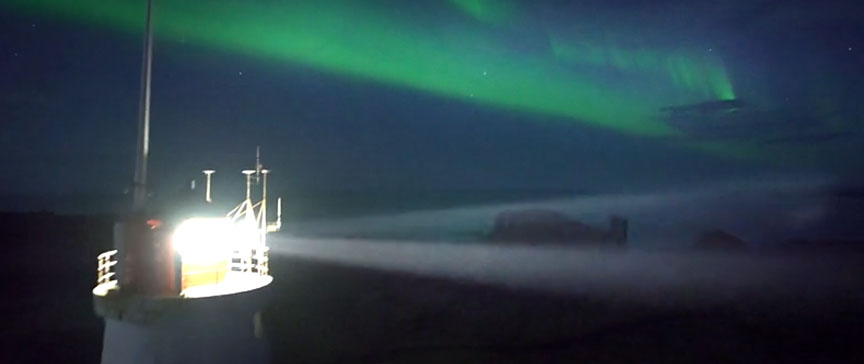
Northern lights over Iceland filmed by Icelandic photographer Oli Haukur using a drone. Don’t forget to expand the screen.
I knew the era of real-time northern lights video was upon us. I just didn’t think drones would get into the act this soon. What was I thinking? They’re perfect for the job! If watching the aurora ever made you feel like you could fly, well now you can in Oli Haukur’s moving, real-time footage of an amazing aurora display filmed by drone.
Oli Haukur operates the drone and camera during a test run. Credit: Oli Hauku / OZZO Photography
Haukur hooked up a Sony a7S II digital camera and ultra-wide Sigma 20mm f/1.4 lens onto his DJI Matrice 600 hexacopter. The light from the gibbous moon illuminates the rugged shoreline and crashing waves of the Reykjanes Peninsula (The Steamy Peninsula) as while green curtains of aurora flicker above.
The Sony camera is shown attached to the drone. To capture the aurora, Haukur used a fast lens, high ISO and set the frame rate to 25 frames per second (fps) or 1/25th of a second per frame. Credit: Oli Haukur / OZZO Photography
When the camera ascends over a sea stack, you can see gulls take off below, surprised by the mechanical bird buzzing just above their heads. Breathtaking. You might notice at the same time a flash of light — this is from the lighthouse beacon seen earlier in the video.
To capture his the footage, Haukur used a “fast” lens (one that needs only a small amount of light to make a picture) and an ISO of 25,600. The camera is capable of ISO 400,000, but the lower ISO provided greater resolution and color quality.
Moonlight provided all the light needed to bring out the landscape.
The drone used to make the night flight and aurora recording is seen up close on takeoff. Haukur, of Rejkyavik, Iceland, works as a freelance photographer and filmmaker as well as providing professional drone services in that country. Credit: Oli Haukur / OZZO Photography
Remember when ISO 1600 or 3200 was as far you dared to go before the image turned to a grainy mush? Last year Canon released a camera that can literally see in the dark with a top ISO over 4,000,000! There’s no question we’ll be seeing more live aurora and drone aurora video in the coming months. Haukur plans additional shoots this winter and early next spring. Living in Iceland, which lies almost directly beneath the permanent auroral oval, you can schedule these sort of things!
Am I allowed one tiny criticism? I want more — a minute and a half is barely enough! Haukur shot plenty but released only a taste to social media to prove it could be done and share the joy. Let’s hope he compiles the rest and makes it available for us to lose our selves in soon.
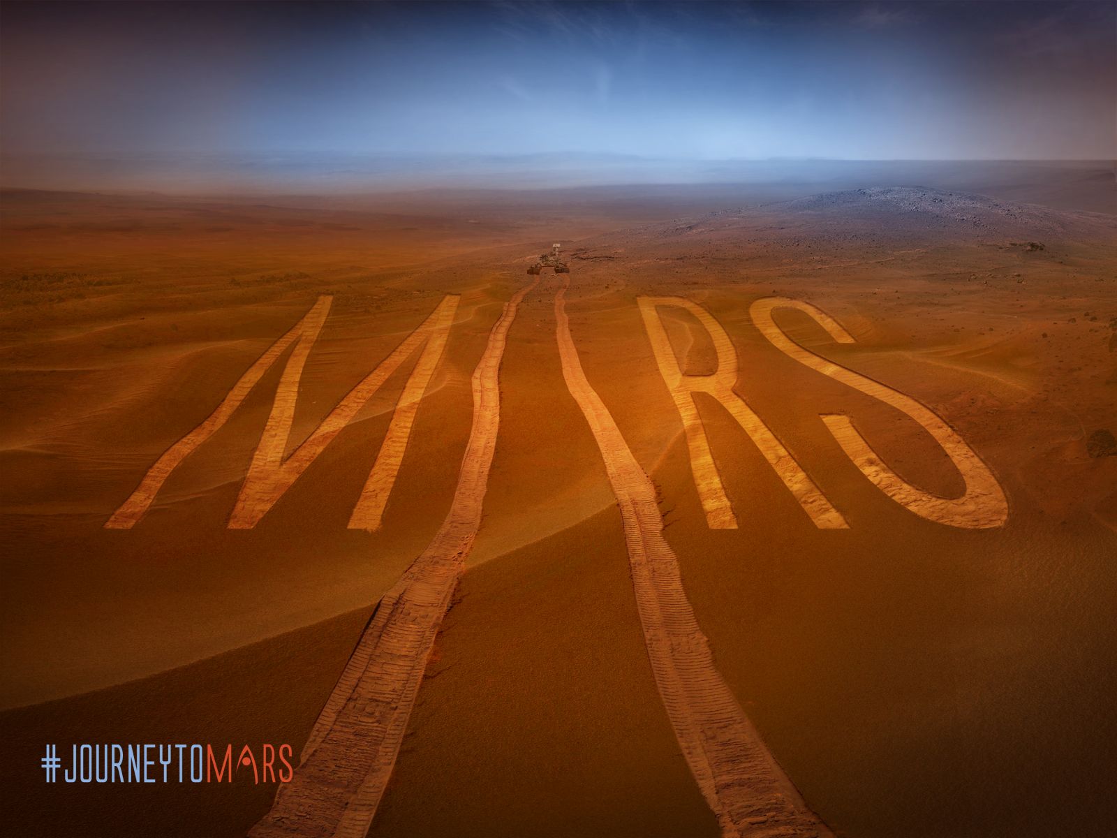
The deployment of the Mars 2020 rover will be the next step in their "Journey to Mars". Credit: NASA
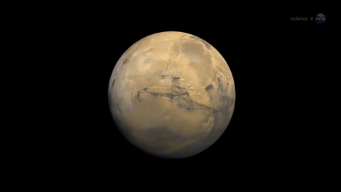
NASA’s Mars Exploration Program has accomplished some truly spectacular things in the past few decades. Officially launched in 1992, this program has been focused on three major goals: characterizing the climate and geology of Mars, looking for signs of past life, and preparing the way for human crews to explore the planet.
And in the coming years, the Mars 2020 rover will be deployed to the Red Planet and become the latest in a long line of robotic rovers sent to the surface. In a recent press release, NASA announced that it has awarded the launch services contract for the mission to United Launch Alliance (ULA) – the makers of the Atlas V rocket.
The mission is scheduled to launch in July of 2020 aboard an Atlas V 541 rocket from Cape Canaveral in Florida, at a point when Earth and Mars are at opposition. At this time, the planets will be on the same side of the Sun and making their closest approach to each other in four years, being just 62.1 million km (38.6 million miles) part.
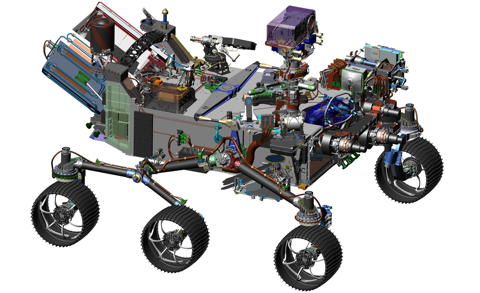
The design of NASA’s Mars 2020 rover combines proven features with some new science instruments and a sampling system. Credits: NASA
Following in the footsteps of the Curiosity, Opportunity andSpirit rovers, the goal of Mars 2020 mission is to determine the habitability of the Martian environment and search for signs of ancient Martian life. This will include taking samples of soil and rock to learn more about Mars’ “watery past”.
But whereas these and other members of the Mars Exploration Program were searching for evidence that Mars once had liquid water on its surface and a denser atmosphere (i.e. signs that life could have existed), the Mars 2020 mission will attempt to find actual evidence of ancient microbial life.
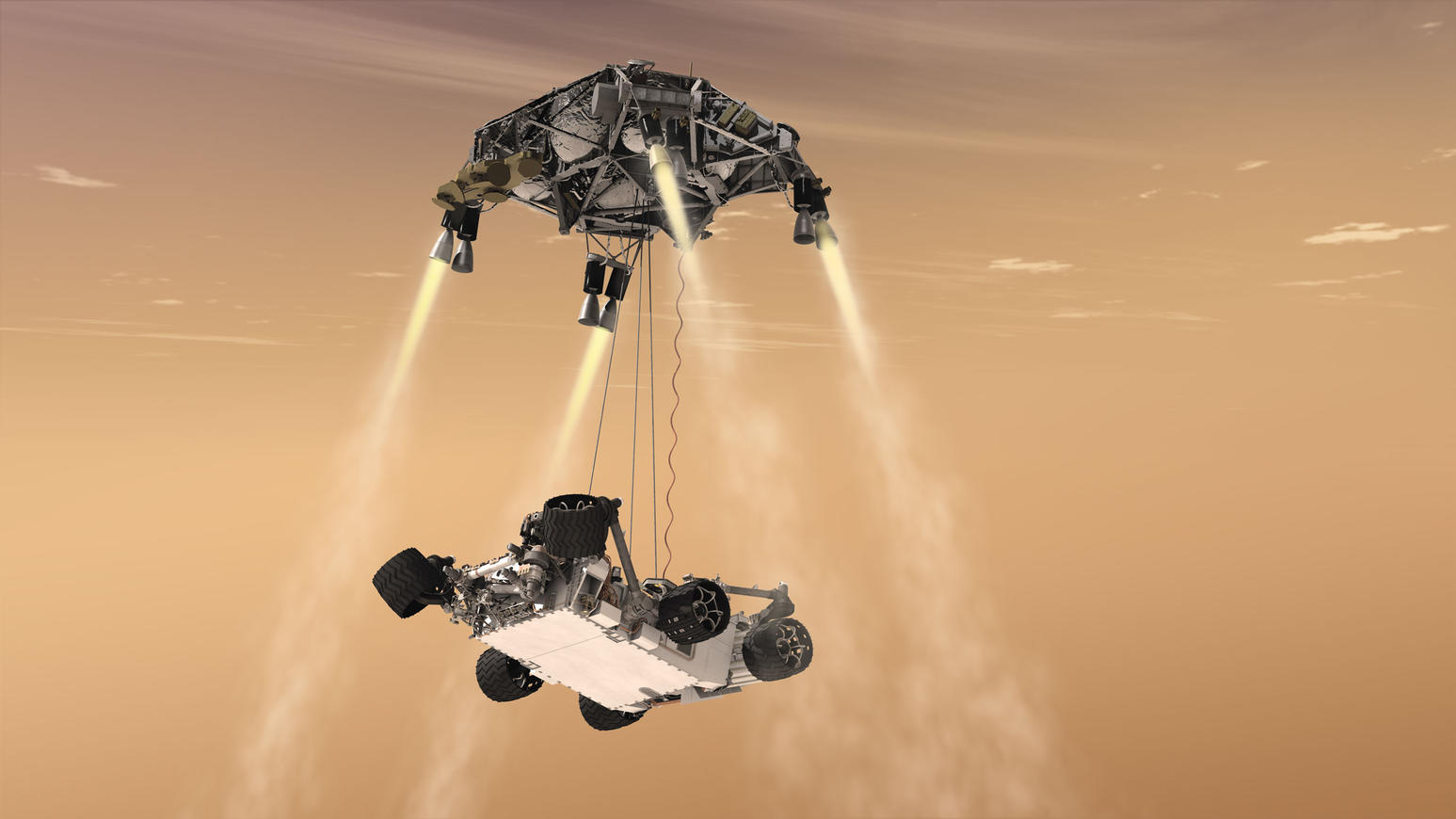
The design of the rover also incorporates several successful features of Curiosity. For instance, the entire landing system (which incorporates a sky crane and heat shield) and the rover’s chassis have been recreated using leftover parts that were originally intended for Curiosity.
There’s also the rover’s radioisotope thermoelectric generator – i.e. the nuclear motor – which was also originally intended as a backup part for Curiosity. But it will also have several upgraded instrument on board that allow for a new guidance and control technique. Known as “Terrain Relative Navigation”, this new landing method allows for greater maneuverability during descent.
Artist’s impression of the Mars 2020, with its sky crane landing system deployed. Credit: NASA/Mars Science Laboratory
Another new feature is the rover’s drill system, which will collect core samples and store them in sealed tubes. These tubes will then be left in a “cache” on the surface, where they will be retrieved by future missions and brought back to Earth – which will constitute the first sample-return mission from the Red Planet.
In this respect, Mars 2020 will help pave the way for a crewed mission to the Red Planet, which NASA hopes to mount sometime in the 2030s. The probe will also conduct numerous studies designed to improve landing techniques and assess the planet’s natural resources and hazards, as well as coming up with methods to allow astronauts to live off the environment.
In terms of hazards, the probe will be looking at Martian weather patterns, dust storms, and other potential environmental conditions that will affect human astronauts living and working on the surface. It will also test out a method for producing oxygen from the Martian atmosphere and identifying sources of subsurface water (as a source of drinking water, oxygen, and hydrogen fuel).
As NASA stated in their press release, the Mars 2020 mission will “offer opportunities to deploy new capabilities developed through investments by NASA’s Space Technology Program and Human Exploration and Operations Mission Directorate, as well as contributions from international partners.”
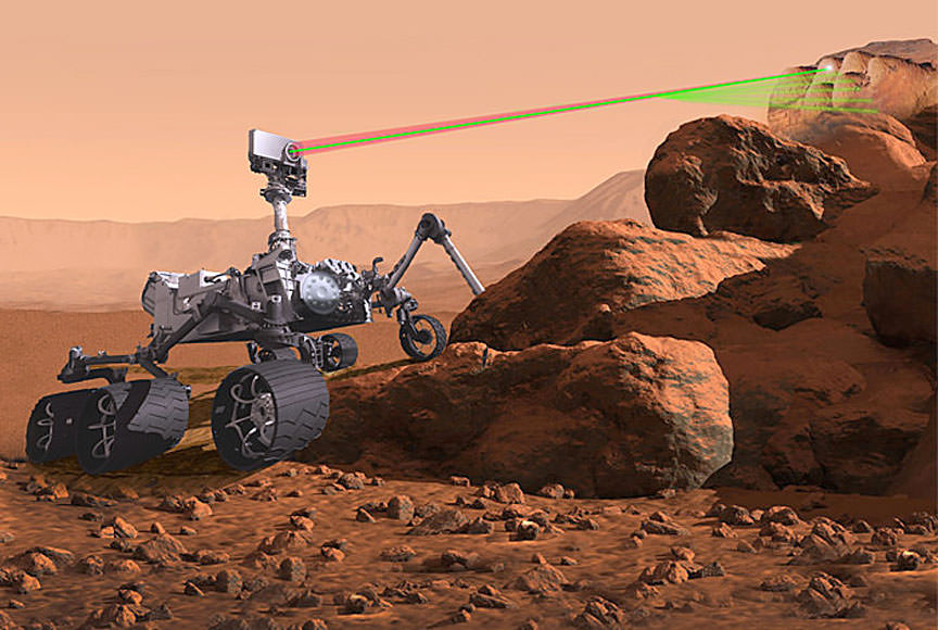
Illustration of the Mars 2020 mission zapping a rock with its laser. Credit: NASA/JPL-
They also emphasized the opportunities to learn ho future human explorers could rely on in-situ resource utilization as a way of reducing the amount of materials needed to be shipped – which will not only cut down on launch costs but ensure that future missions to the planet are more self-reliant.
The total cost for NASA to launch Mars 2020 is approximately $243 million. This assessment includes the cost of launch services, processing costs for the spacecraft and its power source, launch vehicle integration and tracking, data and telemetry support.
The use of spare parts has also meant reduced expenditure on the overall mission. In total, the Mars 2020 rover and its launch will cost and estimated $2.1 billion USD, which represents a significant savings over previous missions like the Mars Science Laboratory – which cost a total of $2.5 billion USD.
Between now and 2020, NASA also intends to launch the Interior Exploration using Seismic Investigations, Geodesy and Heat Transport (InSight) lander mission, which is currently targeted for 2018. This and the Mars 2020 rover will be the latest in a long line of orbiters, rovers and landers that are seeking to unlock the mysteries of the Red Planet and prepare it for human visitors!
Astronaut Jeff Williams just established a new record for most time spent in space by a NASA astronaut. Credit: NASA
The International Space Station has provided astronauts and space agencies with immense opportunities for research during the decade and a half that it has been in operation. In addition to studies involving meteorology, space weather, materials science, and medicine, missions aboard the ISS has also provided us with valuable insight into human biology.
For example, studies conducted aboard the ISS’ have provided us with information about the effects of long-term exposure to microgravity. And all the time, astronauts are pushing the limits of how long someone can healthily remain living under such conditions. One such astronauts is Jeff Williams, the Expedition 48 commander who recently established a new record for most time spent in space.
This record-breaking feat began back in 2000, when Williams spent 10 days aboard the Space Shuttle Atlantis for mission STS-101. At the time, the International Space Station was still under construction, and as the mission’s flight engineer and spacewalker, Williams helped prepare the station for its first crew.
Station Commander Jeff Williams passed astronaut Scott Kelly, also a former station commander, on Aug. 24, 2016, for most cumulative days living and working in space by a NASA astronaut. Credit: NASA
This was followed up in 2006, where Williams’ served as part of Expedition 13 to the ISS. The station had grown significantly at this point with the addition of Russian Zvezda service module, the U.S. Destiny laboratory, and the Quest airlock. Numerous science experiments were also being conducted at this time, which included studies into capillary flow and the effects of microgravity on astronauts’ central nervous systems.
During the six months he was aboard the station, Williams was able to get in two more spacewalks, set up additional experiments on the station’s exterior, and replaced equipment. Three years later, he would return to the station as part of Expedition 21, then served as the commander of Expedition 22, staying aboard the station for over a year (May 27th, 2009 to March 18th, 2010).
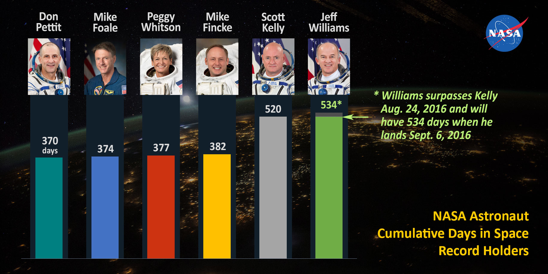
By the time Expedition 48’s Soyuz capsule launched to rendezvous with the ISS on July 7th, 2016, Williams had already spent more than 362 days in space. By the time he returns to Earth on Sept. 6th, he will have spent a cumulative total of 534 days in space. He will have also surpassed the previous record set by Scott Kelly, who spent 520 days in space over the course of four missions.
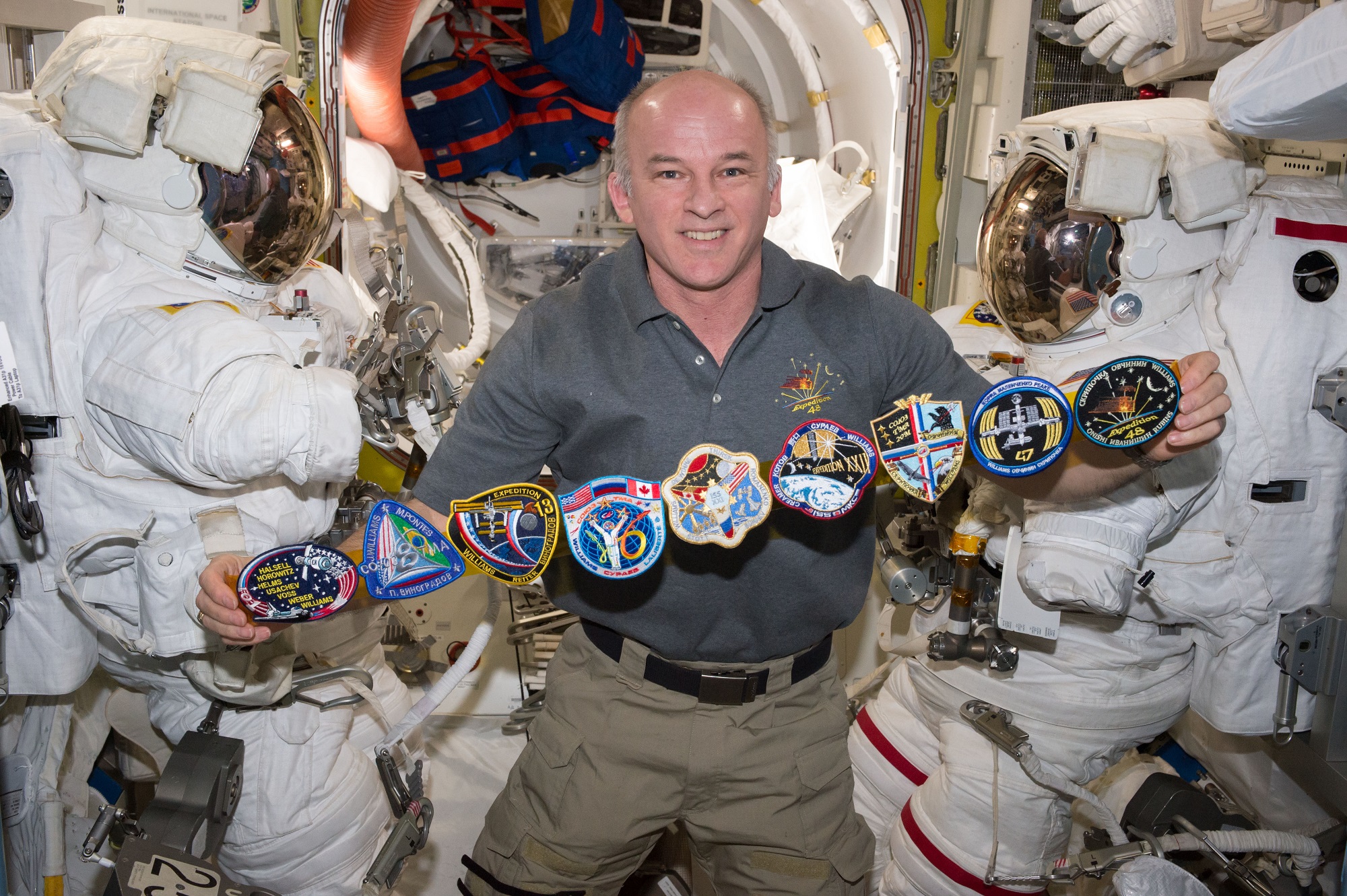
Expedition 48 crew portrait with 46S crew (Jeff Williams, Oleg Skripochka, Aleksei Ovchinin) and 47S crew (Anatoli Ivanishin, Kate Rubins, Takuya Onishi). Credit: NASA
On Wednesday, August 24th, the International Space Station raised its orbit ahead of Williams’ departure. Once he and two of his mission colleagues – Oleg Skripochka and Alexey Ovchinin – undock in their Soyuz TMA-20M spacecraft, they begin their descent towards Kazakhstan, arriving on Earth roughly three and a half hours later.
Former astronaut Scott Kelly was a good sport about the passing of this record, congratulating Williams in a video created by the Johnson Space Center (see below). Luckily, Kelly still holds the record for the longest single spaceflight by a NASA astronaut – which lasted a stunning 340 days.
And Williams may not hold the record for long, as astronaut Peggy Whitson is scheduled to surpass him in 2017 during her next mission (which launches this coming November). And as we push farther out into space in the coming years, mounting missions to NEOs and Mars, this record is likely to be broken again and again.
NASA’s Journey to Mars. NASA is developing the capabilities needed to send humans to an asteroid by 2025 and Mars in the 2030s. Credit: NASA/JPL
In the meantime, Williams and his crew will continue to dedicate their time to a number of crucial experiments. In the course of this mission, they have conducted research into human heart function, plant growth in microgravity, and executed a variety of student-designed experiments.
Like all research conducted aboard the ISS, the results of this research will be used to improve health treatments, have numerous industrial applications here on Earth, and will help NASA plan mission farther into space. Not the least of which will be NASA’s proposed (and rapidly approaching) crewed mission to Mars.
In addition to spending several months in zero-g for the sake of the voyage, NASA will need to know how their astronauts will fair when conducting research on the surface of Mars, where the gravity is roughly 37% that of Earth (0.376 g to be exact).
And be sure to enjoy this video of Scott Kelly congratulating Williams on his accomplishment, courtesy of the Johnson Space Center:
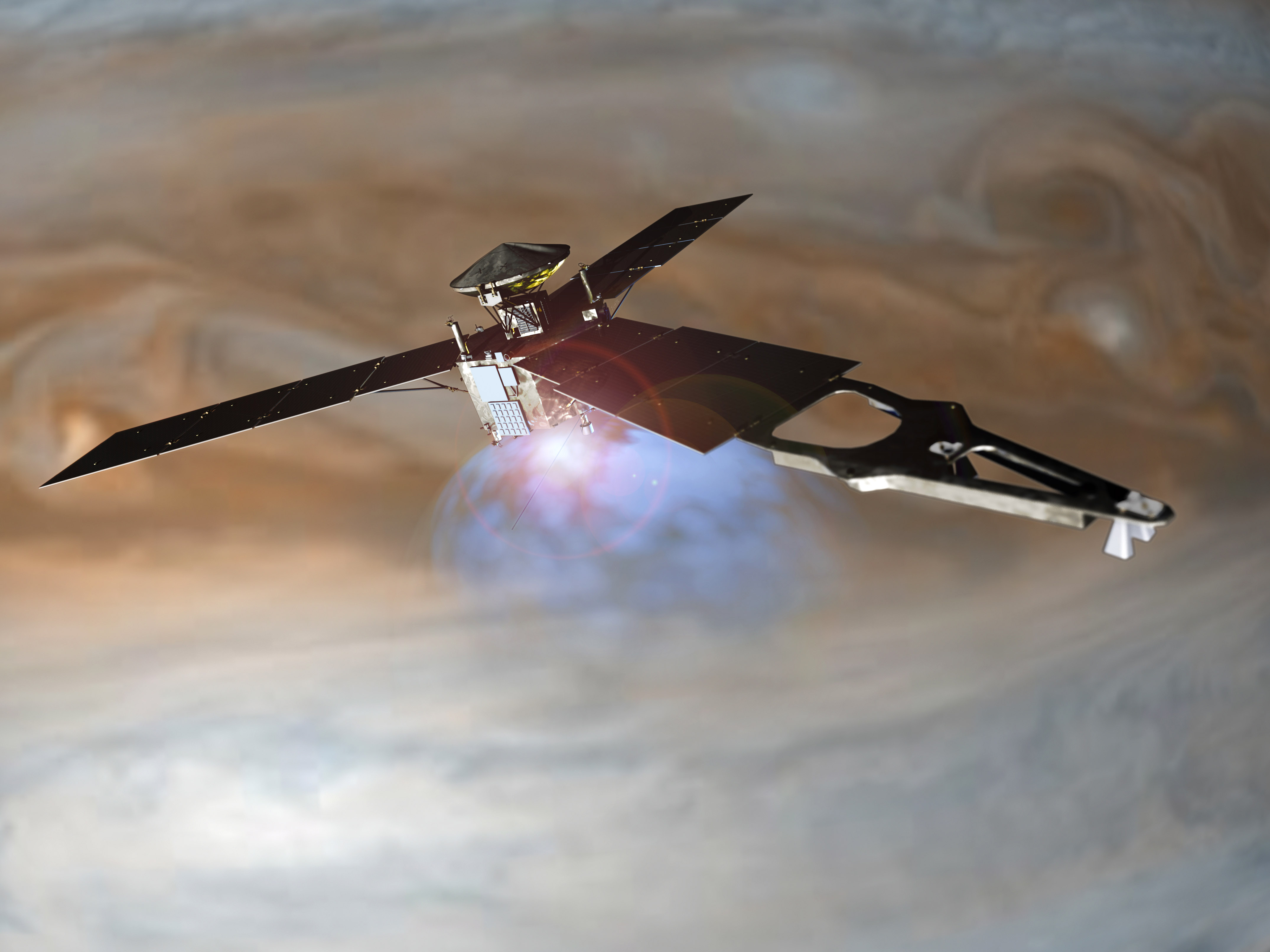
Illustration of NASA's Juno spacecraft firing its main engine to slow down and go into orbit around Jupiter. Lockheed Martin built the Juno spacecraft for NASA's Jet Propulsion Laboratory. Credit: NASA/Lockheed Martin
The Juno spacecraft made history on July 4th, 2016, when it became the second spacecraft in history to achieve orbit around Jupiter for the sake of a long-term mission. Following in the footsteps of the Galileo mission, the probe will spend the next 20 months gathering data on Jupiter’s atmosphere, clouds, interior and gravitational and magnetic fields, before purposefully crashing into the planet.
And on Saturday, August 27th, Juno will be making history once again. According to NASA, at precisely 12:51 UTC (5:51 a.m. PDT, 8:51 a.m. EDT) the spacecraft will be passing closer to the cloud tops of Jupiter than at any point in its main mission. And while the probe is expected to make 35 more close flybys of the gas giant before its mission ends in February of 2018, this particular one is expected to be especially revealing.
For one, it will be the first time that the probe has all of its scientific instruments online and surveying Jupiter’s atmosphere as it swings past. And during the flyby, the probe will be passing Jupiter’s cloud tops at a distance of 4,200 kilometers (2,500 miles) – closer than it will ever get again – while traveling at a speed of 208,000 km/hour (130,000 mph).
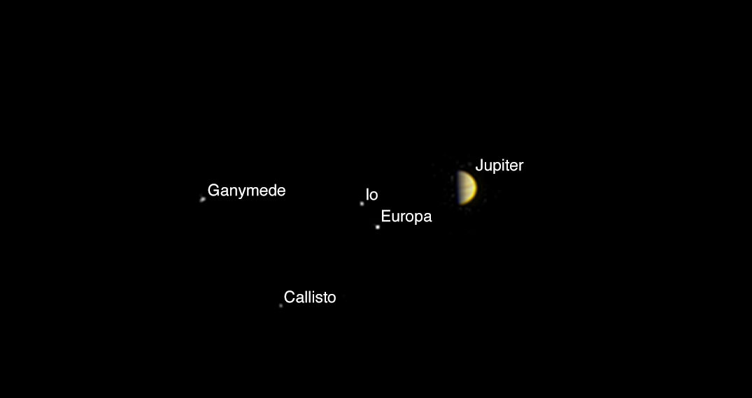
This annotated color view of Jupiter and its four largest moons — Io, Europa, Ganymede and Callisto — was taken by the JunoCam camera on NASA’s Juno spacecraft on June 21, 2016, at a distance of 6.8 million miles (10.9 million kilometers) from Jupiter. Image credit: NASA/JPL-Caltech/MSSS
This will not only be the closest approach to Jupiter made by any probe, but it will pass over Jupiter’s poles, which will give Juno the opportunity to get a look at some never-before-seen things. These will include infrared and microwave readings taken by Juno’s suite of eight instruments, but also some choice photographs.
Yes, in addition to its sensor package, Juno‘s visible light imager (aka. JunoCam) will also be active and taking some close-up pictures of the atmosphere and poles. While the scientific information is expected to keep NASA scientists occupied for some time to come, the JunoCam images are expected to be released later next week.
According to NASA, these images will be the highest resolution photos of the Jovian atmosphere ever taken, not to mention the first glimpse of Jupiter’s north and south poles ever. As Scott Bolton, principal investigator of Juno from the Southwest Research Institute in San Antonio, said in a NASA press release:
“This is the first time we will be close to Jupiter since we entered orbit on July 4. Back then we turned all our instruments off to focus on the rocket burn to get Juno into orbit around Jupiter. Since then, we have checked Juno from stem to stern and back again. We still have more testing to do, but we are confident that everything is working great, so for this upcoming flyby Juno’s eyes and ears, our science instruments, will all be open… This is our first opportunity to really take a close-up look at the king of our Solar System and begin to figure out how he works.”
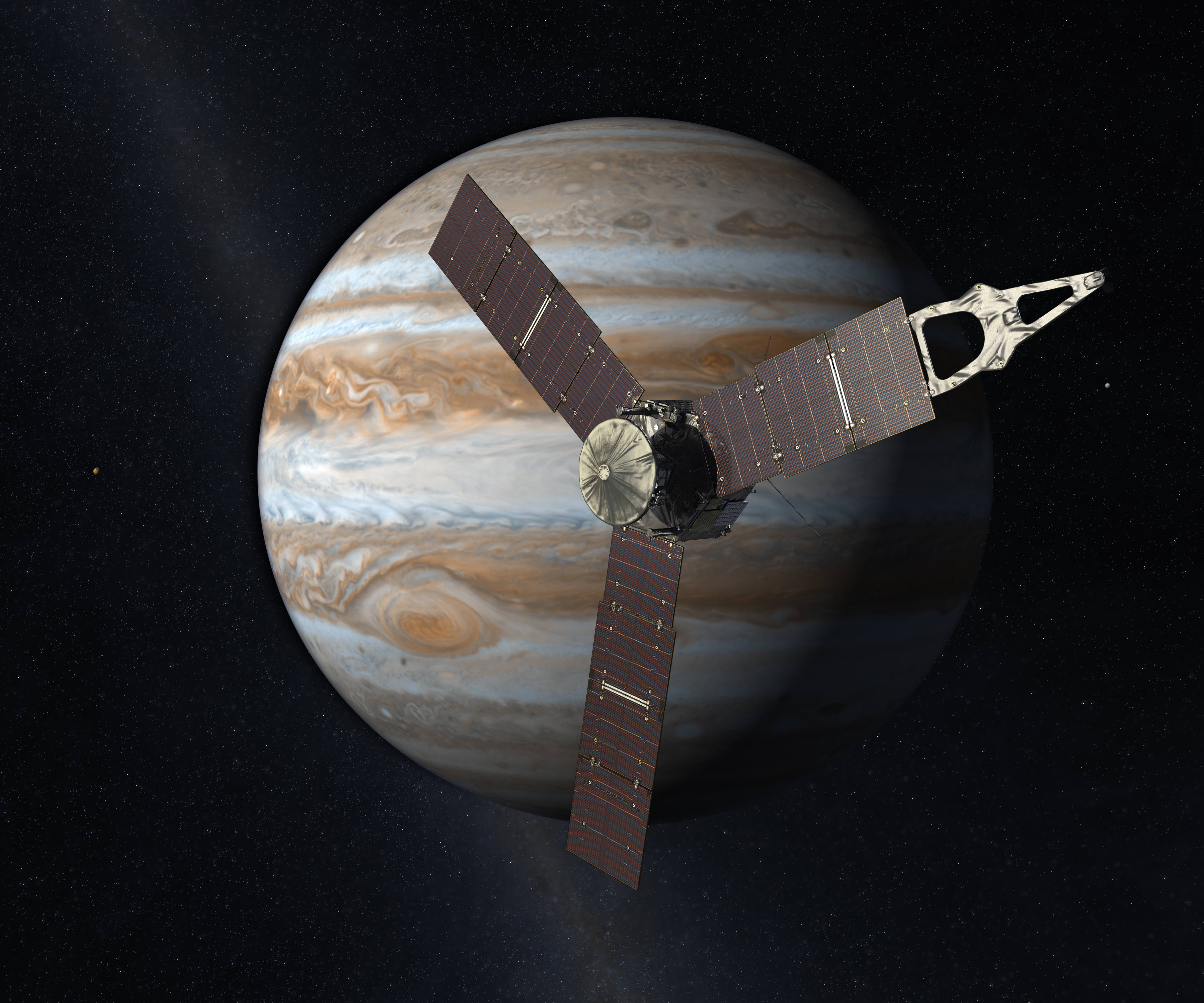
NASA’s Juno spacecraft launched on August 6, 2011 and should arrive at Jupiter on July 4, 2016. Credit: NASA / JPL
Ever since the Juno spacecraft launched on Aug. 5th, 2011, from Cape Canaveral, Florida, scientists and astronomers have been waiting for the day when it would start sending back information on the Solar System’s greatest planet. By examining the atmosphere, interior, and magnetic environment of the gas giant, scientists hope to be able to answer burning questions about the history of the planet’s formation.
For example, Jupiter’s interior structure and composition, as well as what drives its magnetic field, are still the subject of debate. In addition, there are some unanswered questions about when and where the planet formed. While it may have formed in its current orbit, some evidence suggests that it could have formed farther from the sun before migrating inward. All of these questions, it is hoped, are things the Juno mission will answer.
In so doing, scientists hope to be able to shed some additional light on the history of the Solar System as well. Like the other gas giants, it was assembled during the early phases, before our Sun had the chance to absorb or blow away the light gases in the huge cloud from which both were born. As such, Jupiter’s composition could tell us much about the early Solar System.
And this Saturday, the probe will be gathering what could prove to be the most crucial information its mission will produce. And of course, if all goes well, it will be taking the most detailed pictures of the Jovian giant to date! Godspeed, little Juno. You be careful out there!
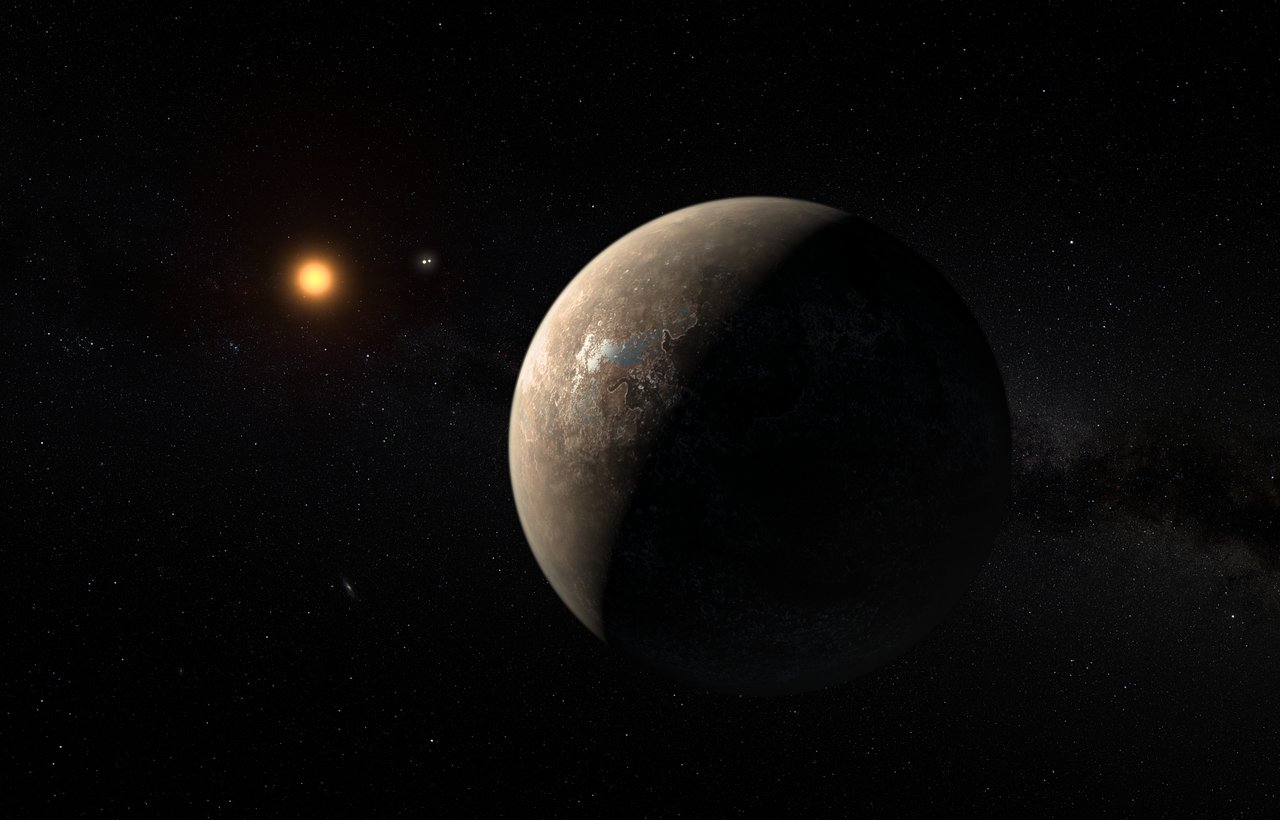
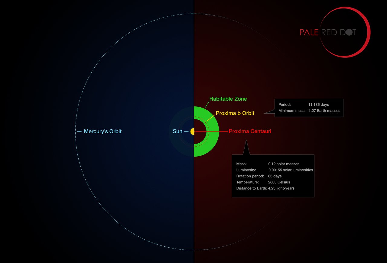
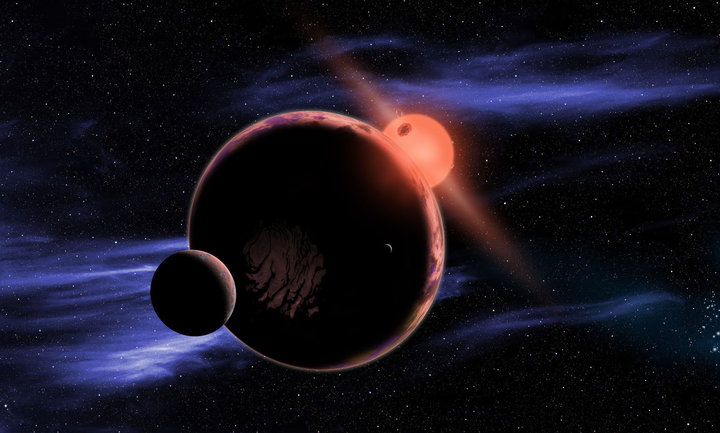
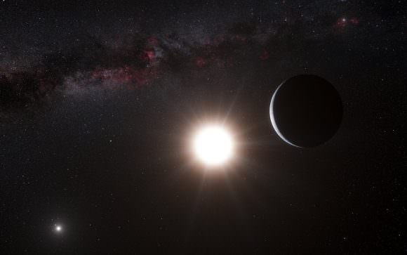
Artist’s impression of the surface of the planet Proxima b orbiting the red dwarf star Proxima Centauri. The double star Alpha Centauri AB is visible to the upper right of Proxima itself. Credit: ESO
The ESO’s recent announcement that they have discovered an exoplanet candidate orbiting Proxima Centauri – thus confirming weeks of speculation – has certainly been exciting news! Not only is this latest find the closest extra-solar planet to our own Solar System, but the ESO has also indicated that it is rocky, similar in size and mass to Earth, and orbits within the star’s habitable zone.
However, in the midst of this news, there has been some controversy regarding certain labels. For instance, when a planet like Proxima b is described as “Earth-like”, “habitable”, and/or “terrestrial“, there are naturally some questions as to what this really means. For each term, there are particular implications, which in turn beg for clarification.
For starters, to call a planet “Earth-like” generally means that it is similar in composition to Earth. This is where the term “terrestrial” really comes into play, as it refers to a rocky planet that is composed primarily of silicate rock and metals which are differentiated between a metal core and a silicate mantle and crust.
This applies to all planets in the inner Solar System, and is often used in order to differentiate rocky exoplanets from gas giants. This is important within the context of exoplanet hunting, as the majority of the 4,696 exoplanet candidates – of which 3,374 have been confirmed (as of August 18th, 2016) – have been gas giants.
What this does not mean, at least not automatically, is that the planet is habitable in the way Earth is. Simply being terrestrial in nature is not an indication that the planet has a suitable atmosphere or a warm enough climate to support the existence of liquid water or microbial life on its surface.
What’s more, Earth-like generally implies that a planet will be similar in mass and size to Earth. But this is not the same as composition, as many exoplanets that have been discovered have been labeled as “Earth-sized” or “Super-Earths” – i.e. planets with around 10 times the mass of Earth – based solely on their mass.
This term also distinguishes an exoplanet candidate from those that are 15 to 17 masses (which are often referred to as “Neptune-sized”) and those that have masses similar to, or many times greater than that of Jupiter (i.e. Super-Jupiters). In all these cases, size and mass are the qualifiers, not composition.
Ergo, finding a planet that is greater in size and mass than Earth, but significantly less than that of a gas giant, does not mean it is terrestrial. In fact, some scientists have recommended that the term “mini-Neptune” be used to describe planets that are more massive than Earth, but not necessarily composed of silicate minerals and metals.
And estimates of size and mass are not exactly metrics for determining whether or not a planet is “habitable”. This term is especially sticky when it comes to exoplanets. When scientists attach this word to extra-solar planets like Proxima b, Gliese 667 Cc, Kepler-452b, they are generally referring to the fact that the planet exists within its parent star’s “habitable zone” (aka. Goldilocks zone).
This term describes the region around a star where a planet will experience average surface temperatures that allow for liquid water to exist on its surface. For those planets that orbit too close to their star, they will experience intense heat that transforms surface water into hydrogen and oxygen – the former escaping into space, the latter combining with carbon to form CO².
This is what scientists believe happened to Venus, where thick clouds of CO² and water vapor triggered a runaway greenhouse effect. This turned Venus from a world that once had oceans into the hellish environment we know today, where temperatures are hot enough to melt lead, atmospheric density if off the charts, and sulfuric acid rains from its thick clouds.
Kepler-62f, an exoplanet that is about 40% larger than Earth. It’s located about 1,200 light-years from our solar system in the constellation Lyra. Credit: NASA/Ames/JPL-Caltech
For planets that orbit beyond a star’s habitable zone, water ice will become frozen solid, and the only liquid water will likely be found in underground reservoirs (this is the case on Mars). As such, finding planets that are just right in terms of average surface temperature is intrinsic to the “low-hanging fruit” approach of searching for life in our Universe.
But of course, just because a planet is warm enough to have water on its surface doesn’t mean that life can thrive on it. As our own Solar System beautifully demonstrates, a planet can have the necessary conditions for life, but still become a sterile environment because it lacks a protective magnetosphere.
This is what scientists believe happened to Mars. Located within our Sun’s Goldilocks zone (albeit on the outer edge of it), Mars is believed to have once had an atmosphere and liquid water on its surface. But today, atmospheric pressure on the surface of Mars is only 1% that of Earth’s, and the surface is dry, cold, and devoid of life.
The reason for this, it has been determined, is because Mars lost its magnetosphere 4.2 Billion years ago. According to NASA’s MAVEN mission, this resulted in Mars’ atmosphere being slowly stripped away over the course of the next 500 million years by solar wind. What little atmosphere it had left was not enough to retain heat, and its surface water evaporated.
Billions of years ago, Mars was a very different world. Liquid water flowed in long rivers that emptied into lakes and shallow seas. A thick atmosphere blanketed the planet and kept it warm. Credit: NASA
By the same token, planets that do not have protective magnetospheres are also subject to an intense level of radiation on their surfaces. On the Martian surface, the average dose of radiation is about 0.67 millisieverts (mSv) per day, which is about a fifth of what people are exposed to here on Earth in the course of a year.
We can expect similar situations on extra-solar planets where a magnetosphere does not exist. Essentially, Earth is fortunate in that it not only orbits in a pretty cushy spot around our Sun, but that its core is differentiated between a solid inner core and a liquid, rotating outer core. This rotation, it is believed, is responsible for creating a dynamo effect that in turn creates Earth’s magnetic field.
However, using our own Solar System again as a model, we find that magnetic fields are not entirely uncommon. While Earth is the only terrestrial planet in our Solar System to have on (all the gas giants have powerful fields), Jupiter’s moon Ganymede also has a magnetosphere of its own.
Similarly, there are orbital parameters to consider. For instance, a planet that is similar in size, mass and composition could still have a very different climate than Earth due to its orbit. For one, it may be tidally-locked with its star, which would mean that one side is permanently facing towards it, and is therefore much warmer.
An artist’s depiction of planets transiting a red dwarf star in the TRAPPIST-1 System. Credit: NASA/ESA/STScl
On the other hand, it may have a slow rotational velocity, and a rapid orbital velocity, which means it only experiences a few rotations per orbit (as is the case with Mercury). Last, but certainly not least, its distance from its respective star could mean it receives far more radiation than Earth does – regardless of whether or not it has a magnetosphere.
This is believed to the be the case with Proxima Centauri b, which orbits its red dwarf star at a distance of 7 million km (4.35 million mi) – only 5% of the Earth’s distance from the Sun. It also orbits Proxima Centauri with an orbital period of 11 days, and either has a synchronous rotation, or a 3:2 orbital resonance (i.e. three rotations for every two orbits).
Because of this, the climate is likely to be very different than Earth’s, with water confined to either its sun-facing side (in the case of a synchronous rotation), or in its tropical zone (in the case of a 3:2 resonance). In addition, the radiation it receives from its red dwarf star would be significantly higher than what we are used to here on Earth.
So what exactly does “Earth-like” mean? The short answer is, it can mean a lot of things. And in this respect, its a pretty dubious term. If Earth-like can mean similarities in mass, size, composition, and can allude to the fact that planet orbits within its star’s habitable zone – but not necessarily all of the above – then its not a very reliable term.
Artist’s impression of the Earth-like planets that have been observed in other star systems. Image Credit: JPL
In the end, the only way to keep things clear would be to describe a planet as “Earth-like” if it in fact shows similarities in terms of size, mass and composition, all at the same time. The word “terrestrial” can certainly be substituted in a pinch, but only where the composition of the planet is known with a fair degree of certainty (and not just its size and mass).
And words like “habitable” should probably only be used when chaperoned by words like “potentially”. After all, being within a star’s habitable zone certainly means there’s the potential for life. But it doesn’t not necessarily entail that life could have emerged there, or that humans could live there someday.
And should these words apply to Proxima b? Perhaps, but one should consider the fact that the ESO has announced the detection of a exoplanet using the Radial Velocity method. Until such time as it is confirmed using direct detection methods, its remains a candidate exoplanet (not a confirmed one).
But even these simple measures would likely not be enough to erase all the ambiguity or controversy. When it comes right down to it, planet-hunting – like all aspects of space exploration and science – is a divisive issue. And new findings always have a way of drawing criticism and disagreement from several quarters at once.
And you thought Pluto’s classification confused things! Well, Pluto has got nothing on the exoplanet database! So be prepared for many years of classification debates and controversy!
Artist's impression of a directed-energy propulsion laser sail in action. Credit: Q. Zhang/deepspace.ucsb.edu
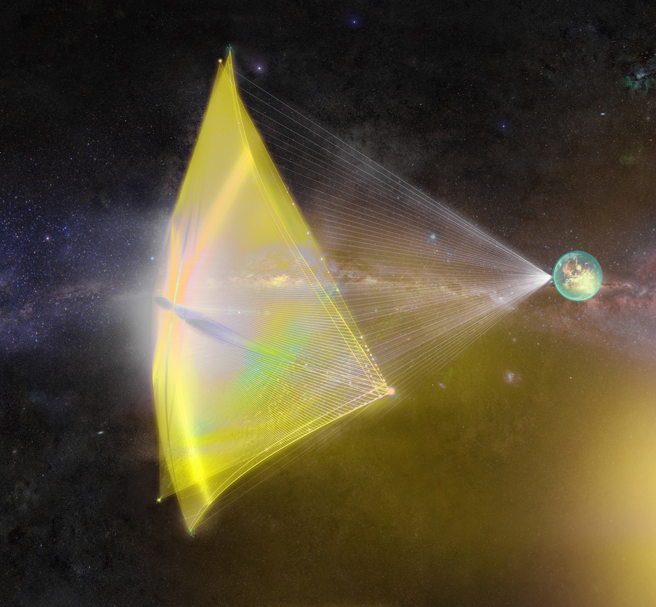
Back in April, Russian billionaire Yuri Milner and famed cosmologist Stephen Hawking unveiled Project Starshot. As the latest venture by Breakthrough Initiatives, Starshot was conceived with the aims of sending a tiny spacecraft to the neighboring star system Alpha Centauri in the coming decades.
Relying on a sail that would be driven up to relativistic speeds by lasers, this craft would theoretically be capable of making the journey is just 20 years. Naturally, this project has attracted its fair share of detractors. While the idea of sending a star ship to another star system in our lifetime is certainly appealing, it presents numerous challenges.
Not one to shy away from any potential problems, Breakthrough Starshot has begun funding the necessary research to make sure that their concept will work. The results of their first research effort appeared recently in arXiv, in a study titled “The interaction of relativistic spacecrafts with the interstellar medium“.
Project Starshot, an initiative sponsored by the Breakthrough Foundation, is intended to be humanity’s first interstellar voyage. Credit: breakthroughinitiatives.org
Assessing the risks of interstellar travel, this paper addresses the greatest threat where relativistic speed is concerned: catastrophic collisions! To put it mildly, space is not exactly an empty medium (despite what the name might suggest). In truth, there are a lot of things out there on the “stellar highway” that can cause a fatal crash.
For instance, within interstellar space, there are clouds of dust particles and even stray atoms of gas that are the result of stellar formations and other processes. Any spacecraft traveling at 20% the speed of light (0.2 c) could easily be damaged or destroyed if it suffered a collision with even the tiniest of this particulate matter.
The research team was led by Dr. Chi Thiem Hoang, a postdoctoral fellow at Canadian Institute for Theoretical Astrophysics (CITA) at the University of Toronto. As Dr. Hoang told Universe Today via email:
“To evaluate the risks, we calculated the energy that each interstellar atom or dust grain transfers to the ship along the path of the projectile in the ship. This acquired energy rapidly heats a spot on the ship surface to high temperature, resulting in damage by reducing the material strength, melting or evaporation.”
The layout of the solar system, including the Oort Cloud, on a logarithmic scale. Credit: NASA
In short, the danger of a collision comes not from the physical impact, but from the energy that is generated due to the fact that the spaceship is traveling so fast. However, what they found was that while collisions with tiny dust grains are very likely, collisions with heavier atoms that can do the most damage would be more rare.
Nevertheless, the damage from so many tiny collisions will certainly add up over time. And it would only take one collision with a larger particle to end the mission. As Dr. Hoang explained:
“We found that the ship would be damaged by collision with heavy atoms and dust grains in the interstellar medium. Heavy atoms, mostly iron can damage the surface to a depth of 0.1mm. More importantly, the surface of the ship is eroded gradually by dust grains, to a depth of about 1mm. The ship may be completely destroyed if encountering a very big dust grain larger than 15micron, although it is extremely rare.”
In terms of damage, what they determined was that each iron atom can produce a damage track of 5 nanometer across, whereas a typical dust silicate grain measuring just 0.1. micron across (and containing about one billion iron atoms) could produce a large crater on the ship’s surface.
A phased laser array, perhaps in the high desert of Chile, propels sails on their journey. Credit: Breakthrough Initiatives.
Over time, the cumulative effect of this damage would pose a major risk for the ship’s survival. As a result, Dr. Hoang and his team recommended that some shielding would need to be mounted on the ship, and that it wouldn’t hurt to “clear the road” a little as well.
“We recommended to protect the ship by putting a shield of about 1 mm thickness made of strong, high melting temperature material like graphite.” he said. “We also suggested to destroy interstellar dust by using part of energy from laser sources.”
These projects, which are being funded by NASA, seek to harness the technology behind directed-energy propulsion to rapidly send missions to Mars and other locations within the Solar System in the future. Long-term applications include interstellar missions, similar to Starshot.
Artist’s impression of the Earth-like exoplanet discovered orbiting Alpha Centauri B iby the European Southern Observatory on October 17, 2012. Credit: ES
Other interesting projects overseen by Lubin and the UCSB lab include the Directed Energy System for Targeting of Asteroids and exploRation (DE-STAR). This system calls for the use of lasers to deflect asteroids, comets, and other near-Earth objects (NEO) that pose a credible risk of impact.
In all cases, directed-energy technology is being proposed as the solution to the problems posed by space travel. In the case of Starshot, these include (but are not limited to) inefficiency, mass, and/or the limited speeds of conventional rockets and ion engines.
As Professor Lubin told Universe Today via email, he and his colleagues are in general agreement with the research team and their findings:
“The recent paper by Hoang et al revisits the section (7) in our paper “A Roadmap to Interstellar Flight” that discusses our calculation for the effects of the ISM on the wafer scale spacecraft. Their general conclusion on the effects of the gas and dust collisions were essentially the same as ours, namely that it is an issue, but not a fatal one, if one uses the spacecraft geometry we recommend in our paper, namely orient the spacecraft edge on (like a Frisbee in flight) and then use an edge coating (we use [Beryllium], they use graphite).”
“As for the sail interactions with the ISM we recommend either rotating the sail so it is edge on (lower cross section) or ejecting the sail after the initial few minutes of acceleration as it is no longer needed for acceleration. However. as we desire to use the sail as a reflector for the laser communications we prefer to keep it, though a secondary reflector could be deployed later in the mission if necessary. These detailed questions will be part of the evolving design phase.”
Indeed, there are many safety hazards that have to be accounted for before any mission to interstellar space could be mounted. But as this recent study has shown – with which Professor Lubin agrees – they are not insurmountable, and a mission to Alpha Centauri (or, fingers crossed, Proxima Centauri!) could be performed if the proper precautions are taken.
Who knew the future of space travel would be every bit as cool as we’ve been led to believe – complete with lasers and shielding?
And be sure to enjoy this video from NASA 360, addressing directed-energy propulsion:
Artist’s impression of Proxima b, which was discovered using the Radial Velocity method. Credit: ESO/M. Kornmesser
For years, astronomers have been observing Proxima Centauri, hoping to see if this red dwarf has a planet or system of planets around it. As the closest stellar neighbor to our Solar System, a planet here would also be our closest planetary neighbor, which would present unique opportunities for research and exploration.
So there was much excitement when, earlier this month, an unnamed source claimed that the ESO had spotted an Earth-sized planet orbiting within the star’s habitable zone. And after weeks of speculation, with anticipation reaching its boiling point, the ESO has confirmed that they have found a rocky exoplanet around Proxima Centauri – known as Proxima b.
Located just 4.25 light years from our Solar System, Proxima Centauri is a red dwarf star that is often considered to be part of a trinary star system – with Alpha Centauri A and B. For some time, astronomers at the ESO have been observing Proxima Centauri, primarily with telescopes at the La Silla Observatory in Chile.
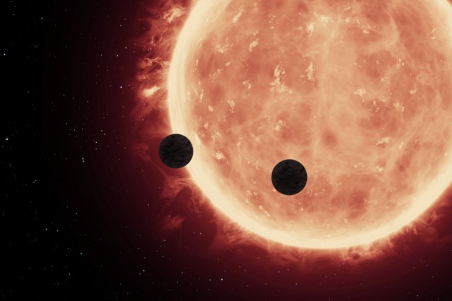
Their interest in this star was partly due to recent research that has shown how other red dwarf stars have planets orbiting them. These include, but are not limited to, TRAPPIST-1, which was shown to have three exoplanets with sizes similar to Earth last year; and Gliese 581, which was shown to have at least three exoplanets in 2007.
The ESO also confirmed that the planet is potentially terrestrial in nature (i.e. rocky), similar in size and mass to Earth, and orbits its star with an orbital period of 11 days. But best of all are the indications that surface temperatures and conditions are likely suitable for the existence of liquid water.
It’s discovery was thanks to the Pale Red Dot campaign, a name which reflects Carl Sagan’s famous reference to the Earth as a “pale blue dot”. As part of this campaign, a team of astronomers led by Guillem Anglada-Escudé – from Queen Mary University of London – have been observing Proxima Centauri for signs of wobble (i.e. the Radial Velocity Method).
After combing the Pale Red Dot data with earlier observations made by the ESO and other observatories, they noted that Proxima Centauri was indeed moving. With a regular period of 11.2 days, the star would vary between approaching Earth at a speed of 5 km an hour (3.1 mph), and then receding from Earth at the same speed.
Artist’s impression of the surface of the planet Proxima b orbiting the red dwarf star Proxima Centauri. The double star Alpha Centauri AB is visible to the upper right of Proxima itself. Credit: ESO
This was certainly an exciting result, as it indicated a change in the star’s radial velocity that was consistent with the existence of a planet. Further analysis showed that the planet had a mass at least 1.3 times that of Earth, and that it orbited the star at a distance of about 7 million km (4.35 million mi) – only 5% of the Earth’s distance from the Sun.
The discovery of the planet was made possible by the La Silla’s regular observation of the star, which took place star between mid-January and April of 2016, using the 3.6-meter telescope‘s HARPS spectrograph. Other telescopes around the world conducted simultaneous observation in order to confirm the results.
One such observatory was the San Pedro de Atacama Celestial Explorations Observatory in Chile, which relied on its ASH2 telescope to monitor the changing brightness of the star during the campaign. This was essential, as red dwarfs like Proxima Centauri are active stars, and can vary in ways that would mimic the presence of the planet.
Guillem Anglada-Escudé described the excitement of the past few months in an ESO press release:
“I kept checking the consistency of the signal every single day during the 60 nights of the Pale Red Dot campaign. The first 10 were promising, the first 20 were consistent with expectations, and at 30 days the result was pretty much definitive, so we started drafting the paper!”
Infographic comparing the orbit of the planet around Proxima Centauri (Proxima b) with the same region of the Solar System. Credit: ESO/M. Kornmesser/G. Coleman
Two separate papers discuss the habitability of Proxima b and its climate, both of which will be appearing soon on the Institute of Space Sciences (ICE) website. These papers describe the research team’s findings and outline their conclusions on how the existence of liquid water cannot be ruled out, and discuss where it is likely to be distributed.
Though there has been plenty of excitement thanks to words like “Earth-like”, “habitable zone”, and “liquid water” being thrown around, some clarifications need to be made. For instance, Proxima b’s rotation, the strong radiation it receives from its star, and its formation history mean that its climate is sure to be very different from Earth’s.
For instance, as is indicated in the two papers, Proxima b is not likely to have seasons, and water may only be present in the sunniest regions of the planet. Where those sunny regions are located depends entirely on the planet’s rotation. If, for example, it has a synchronous rotation with its star, water will only be present on the sun-facing side. If it has a 3:2 resoncance rotation, then water is likely to exist only in the planet’s tropical belt.
In any case, the discovery of this planet will open the door to further observations, using both existing instruments and the next-generation of space telescopes. And as Anglada-Escudé states, Proxima Centauri is also likely to become the focal point in the search for extra-terrestrial life in the coming years.
A view of the southern skies over the ESO 3.6-metre telescope at the La Silla Observatory in Chile, showing the location of Proxima Centauri in the sky. Credit: Y. Beletsky (LCO)/ESO/ESA/NASA/M. Zamani
“Many exoplanets have been found and many more will be found, but searching for the closest potential Earth-analogue and succeeding has been the experience of a lifetime for all of us,” he said. “Many people’s stories and efforts have converged on this discovery. The result is also a tribute to all of them. The search for life on Proxima b comes next…”
As we noted in a previous article on the subject, Project Starshot is currently developing a nanocraft that will use a laser-driven sail to make the journey to Alpha Centauri in 20 years time. But a mission to Proxima Centuari would take even less time (19.45 years at the same speed), and could study this newly-found exoplanet up-close.
One can only hope they are planning on altering their destination to take advantage of this discovery. And one can only imagine what they might find if and when they get to Proxima b!
Don't blink... an artist's conception of an asteroid blocking out a distant star. Image credit: NASA.
Up for a challenge? Over the next two weekends, two asteroid occultations pass over North America. These are both occulting (passing in front of) +7th magnitude stars, easy targets for even binoculars or a small telescope. These events both have a probability score of 99-100%, meaning the paths are known to a high degree of accuracy. These are also two of the more high profile asteroid occultations for 2016.
Here’s the lowdown on both events:
The path of the 85 Io event. Image credit: Steve Preston/Asteroid Occultation Updates.
On the morning of Saturday, August 27th , the +10th magnitude asteroid 85 Io occults a +7.5 magnitude star (TYC 0517-00165-1). the maximum predicted duration for the event is 28 seconds, and the maximum predicted brightness drop is expected to be 3 magnitudes. The ‘shadow’ will cross North America from the northeast to the southwest starting over Quebec at 4:27 Universal Time (UT), crossing Ontario and Michigan’s upper peninsula at 4:30 UT, and heading south over Oklahoma, Texas, and Mexico at 4:36 UT. The action takes place in the constellation Aquarius, with the Moon at a 28% waning crescent.
A wide field finder view for the 85 Io event. Image credit: Stellarium
Discovered by C.H.F. Peters on September 19th, 1865, 85 Io is about 180 kilometers in diameter, as measured by an occultation in late 1995.
The path of the 51 Nemausa event. Image credit: Steve Preston/Asteroid occultation updates.
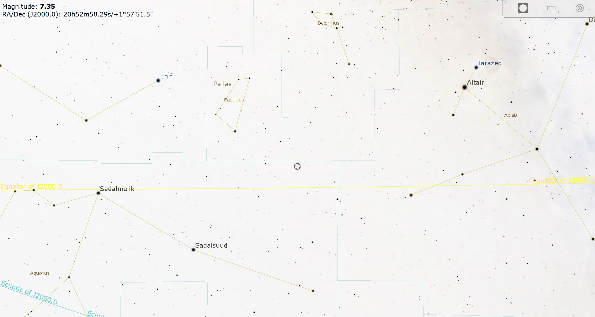
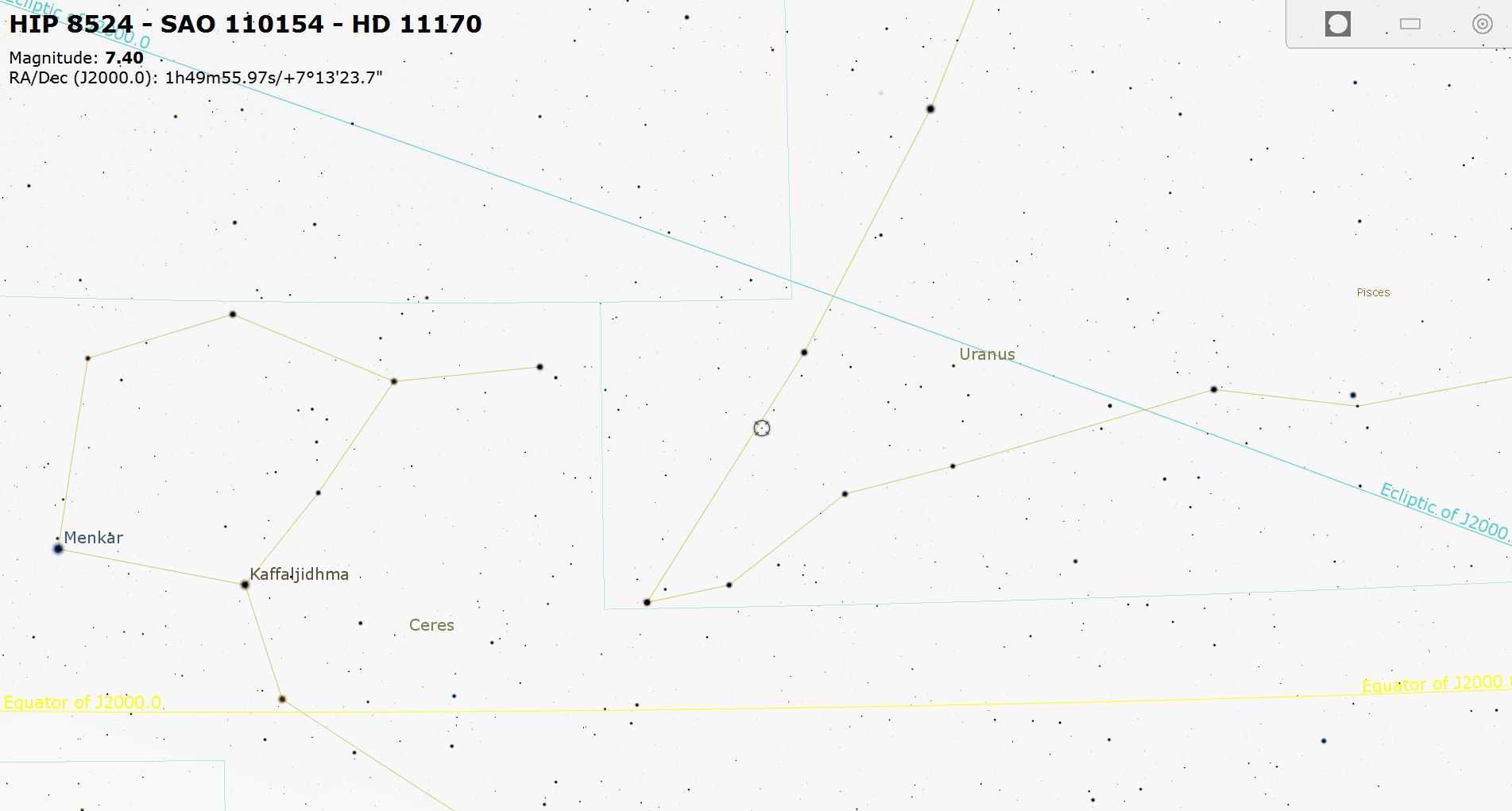
Next, on the morning of Saturday, September 3rd, the +11.5 magnitude asteroid 51 Nemausa occults a +7.6 mag star (HIP 8524). The maximum duration of the event along the centerline is expected to be 32 seconds in duration, with a maximum drop of four magnitudes. Said shadow will cross western Canada at9:42 UT, and the U.S. crossing runs from 9:49 to 9:55 UT. The action takes place in the constellation Pisces. The Moon phase is a slim 4% waxing crescent during the event.
A wide field finder view for the 51 Nemausa event. Image credit: Stellarium
Discovered in 1858 by A. Laurent observing from Nîmes, France, 51 Nemausa occulted a bright star in 1979. In fact, there’s evidence from previous occultation to suggest the 51 Nemausa may possess a tiny moon… could it show up again during the September 3rd event?
Observing asteroid occultations is really a modern sub-specialty of amateur and even professional astronomy. To predict such an occurrence, the orbit of the asteroid or occulting body and the precise position of the star need to be known to a pretty high degree of precision. This required the advent of modern astrometry and massive computing power. If any casual sky observer noticed a naked eye star wink out way back when pre-mid 20th century, it’s lost to history.
The first successfully predicted and observed occultation of a star by an asteroid was the +8.2 magnitude star SAO 112328 by 3 Juno on February 19, 1958. Less than two dozen such events were observed right up through to 1980. Today, hundreds of such events are predicted worldwide each year.
Next month’s expected data release from the ESA’s Gaia mission should refine our stellar position and parallax knowledge even further, and fine-tune predictions of future asteroid occultations.
Observing an asteroid occultation is a challenge, requiring an observer acquiring and monitoring the correct star at the precise time of the event. If possible (i.e. weather permitting) familiarize yourself with the star field a night or two prior to the event. I usually have a precise audio time signal such as WWV radio running in the background.
The shape of 51 Nemausa from the 2014 event. Image credit: Occult 4.2.
Why occultations? Well, if enough observations can be gathered, a sort of shadow profile of the occulting space rock can be made, with each observation representing a chord. Even negative ‘misses’ along the edge of the path help. Tiny moons of asteroids have even been discovered this way, as the distant star winks out multiple times.
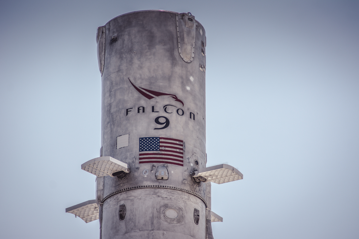
The first stage of the very first Falcon 9 to successfully be recovered now stands as a monument outside of SpaceX's headquarters in Hawthorne, California. Credit: KC Grim
SpaceX has certainly pulled off some successful feats lately. In the past few months, the private aerospace company made its second successful landing on solid ground and its third successful landing at sea with their Falcon 9 rocket. In so doing, they demonstrated that they have achieved the long sought-after dream of reusable rocket technology.
And to celebrate these feats, SpaceX has placed a particularly special first stage on display outside the company headquarters in Hawthorne, California. This particular rocket stage made history about eight months ago (on Dec. 21st, 2015), when it became the first-ever first stage to be recovered in the entire history of spaceflight.
For the sake of this mission, which was the 20th flight conducted by SpaceX using this class of rocket, the Falcon 9 was tasked with delivering 11 Orbcomm-OG2 communications satellites into orbit. After separating, the first stage descended to Earth and became the first rocket stage ever to make a soft landing and recovery.
The top of the Falcon-9 lower stage. Credit: KC Grim
Prior to this flight, SpaceX’s had made two attempts at a vertical landing and booster recovery, both of which ended in failure. The first attempt, which took place in January of 2015, ended when the rocket came close to a successful landing aboard the company’s Autonomous Spaceport Drone Ship (ASDS), but then fell over and exploded.
An investigation determined that failure was due to the rocket’s steering fins running out of hydraulic fluid. The second failed attempt, which took place in April of last year, ended when the rocket stage was mere seconds away from landing on ASDS, but once again fell over and exploded. This time around, the culprit was a failure in one of the rocket stage’s engine throttle valves.
On the third attempt, which took place on Dec. 21st, the Falcon 9 first stage landed a mere ten minutes after launching from Earth. After its descent, it successfully touched down in an upright position on SpaceX’s Landing Zone (LZ-1) at Cape Canaveral Air Force Station.
The success of this recovery was a major milestone for the company, and a breakthrough in the history of space exploration and technology. Little wonder then why the company is choosing to honor it by placing it on display at the Hawthorn facility, where their rocket manufacturing plant is located.
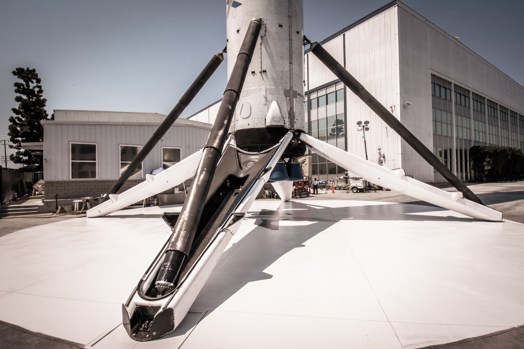
The first stage of the recovered Falcon 9, showing its landing struts deployed. Credit: KC Grim
It all happened this past weekend, where work crews spent Saturday and Sunday standing the 50 meter (165 foot) Falcon 9 stage up on its landing skids. Prior to it being transported to their headquarters in Hawthorne, the rocket’s first stage was being kept in a horizontal position at the NASA Kennedy Space Center in Florida, and then at a location a few blocks away from the HQ.
Getting it to stand again was no easy task, and required two days and two cranes! The rocket also underwent some “aesthetic renewal” before being erected, which included a cleaning in order to remove all the soot it had accumulated on re-entry. Its logos were also repainted, and most of its engines were replaced by spent versions.
Since this first recovery, SpaceX has managed to conduct five more successful recoveries, one on land and four on its ASDS. They are moving ahead with the first launch of their Falcon Heavy – Demo Flight 1, which is scheduled to take place by the end of 2016 – which will be the heaviest rocket to be launched from the US since the retirement of the venerable Saturn V.
Yes, the little company Elon Musk started with the dream of one-day colonizing Mars has certainly achieved some milestones. And between the creation of this display, and the Dragon capsule they have on display inside their Hawthorn headquarters, the company is clearly committed to immortalizing them.
And be sure to enjoy this video of the Falcon 9 making its first successful landing, courtesy of SpaceX:
Artist's renditions of a terrestrial planet orbiting a red dwarf star. Credit: Harvard-Smithsonian Center for Astrophysics (CfA)
For years, exoplanet hunters have been busy searching for planets that are similar to Earth. And when earlier this month, an unnamed source indicated that the European Southern Observatory (ESO) had done just that – i.e. spotted a terrestrial planet orbiting within the star’s habitable zone – the response was predictably intense.
The unnamed source also indicated that the ESO would be confirming this news by the end of August. At the time, the ESO offered no comment. But on the morning of Monday, August 22nd, the ESO broke its silence and announced that it will be holding a press conference this Wednesday, August 24th.
No mention was made as to the subject of the press conference or who would be in attendance. However, it is safe to assume at this point that it’s main purpose will be to address the burning question that’s on everyone’s mind: is there an Earth-analog planet orbiting the nearest star to our own?
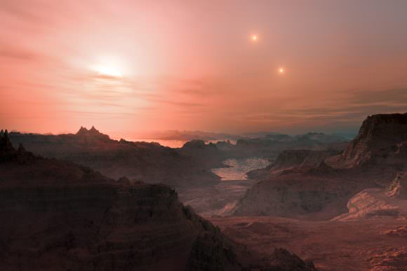
Artist’s impression of a sunset seen from the surface of an Earth-like exoplanet. Credit: ESO/L. Calçada
For years, the ESO has been studying Proxima Centauri using the La Silla Observatory’s High Accuracy Radial velocity Planet Searcher (HARPS). It was this same observatory that reported the discovery of a planet around Alpha Centauri B back in 2012 – which was the “closest planet to Earth” at the time – which has since been cast into doubt.
Relying on a technique known as the Radial Velocity (or Doppler) Method, they have been monitoring this star for signs of movement. Essentially, as planets orbit a star, they exert a gravitational influence of their own which causes the star to move in a small orbit around the system’s center of mass.
Ordinarily, a star would require multiple exoplanets, or a planet of significant size (i.e. a Super-Jupiter) in order for the signs to be visible. In the case of terrestrial planets, which are much smaller than gas giants, the effect on a star’s orbit would be rather negligible. But given that Proxima Centauri is the closest star system to Earth – at a distance of 4.25 light years – the odds of discerning its radial velocity are significantly better.
Artist’s impression of the Earth-like exoplanet discovered orbiting Alpha Centauri B iby the European Southern Observatory on October 17th, 2012. Credit: ESO
According to the source cited by the German weekly Der Speigel, which was the first to report the story, the unconfirmed exoplanet is not only believed to be “Earth-like” (in the sense that it is a rocky body) but also orbits within it’s stars habitable zone (i.e. “Goldilocks Zone”).
Because of this, it would be possible for this planet to have liquid water on its surface, and an atmosphere capable of supporting life. However, we won’t know any of this for certain until we can direct the next-generation of telescopes – like the James Webb Space Telescope or Transiting Exoplanet Survey Satellite (TESS) – to study it more thoroughly.
This is certainly an exciting development, as confirmation will mean that there is planet similar to Earth that is within our reach. Given time and the development of more advanced propulsion systems, we might even be able to mount a mission there to study it up close!
The press conference will start at 1 p.m. Central European Time (CET) – 1 p.m. EDT/10 a.m. PDT. And you bet that we will be reporting on the results shortly thereafter! Stay tuned!