There are a few places in the Universe that defy comprehension. And supernovae have got to be the most extreme places you can imagine. We’re talking about a star with potentially dozens of times the size and mass of our own Sun that violently dies in a faction of a second.
Faster than it take me to say the word supernova, a complete star collapses in on itself, creating a black hole, forming the denser elements in the Universe, and then exploding outward with the energy of millions or even billions of stars.
But not in all cases. In fact, supernovae come in different flavours, starting from different kinds of stars, ending up with different kinds of explosions, and producing different kinds of remnants.
There are two main types of supernovae, the Type I and the Type II. I know this sounds a little counter intuitive, but let’s start with the Type II first.
These are the supernovae produced when massive stars die. We’ve done a whole show about that process, so if you want to watch it now, you can click here.
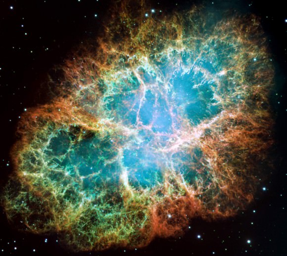
Our eyes would never see the Crab Nebula as this Hubble image shows it. Image credit: NASA, ESA, J. Hester and A. Loll (Arizona State University)
But here’s the shorter version.
Stars, as you know, convert hydrogen into fusion at their core. This reaction releases energy in the form of photons, and this light pressure pushes against the force of gravity trying to pull the star in on itself.
Our Sun, doesn’t have the mass to support fusion reactions with elements beyond hydrogen or helium. So once all the helium is used up, the fusion reactions stop and the Sun becomes a white dwarf and starts cooling down.
But if you have a star with 8-25 times the mass of the Sun, it can fuse heavier elements at its core. When it runs out of hydrogen, it switches to helium, and then carbon, neon, etc, all the way up the periodic table of elements. When it reaches iron, however, the fusion reaction takes more energy than it produces.
The outer layers of the star collapses inward in a fraction of a second, and then detonates as a Type II supernova. You’re left with an incredibly dense neutron star as a remnant.
But if the original star had more than about 25 times the mass of the Sun, the same core collapse happens. But the force of the material falling inward collapses the core into a black hole.
Extremely massive stars with more than 100 times the mass of the Sun just explode without a trace. In fact, shortly after the Big Bang, there were stars with hundreds, and maybe even thousands of times the mass of the Sun made of pure hydrogen and helium. These monsters would have lived very short lives, detonating with an incomprehensible amount of energy. Artist’s impression of a supernova
Those are Type II. Type I are a little rarer, and are created when you have a very strange binary star situation.
One star in the pair is a white dwarf, the long dead remnant of a main sequence star like our Sun. The companion can be any other type of star, like a red giant, main sequence star, or even another white dwarf.
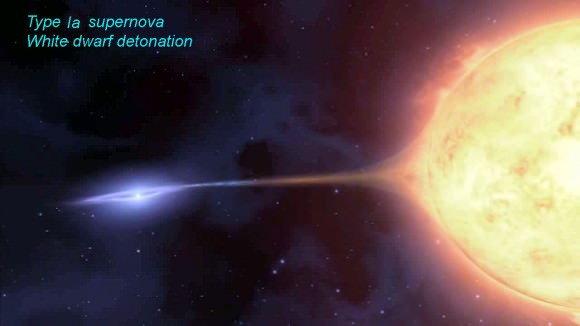
What matters is that they’re close enough that the white dwarf can steal matter from its partner, and build it up like a smothering blanket of potential explosiveness. When the stolen amount reaches 1.4 times the mass of the Sun, the white dwarf explodes as a supernova and completely vaporizes. In a Type Ia supernova, a white dwarf (left) draws matter from a companion star until its mass hits a limit which leads to collapse and then explosion. Credit: NASA
Because of this 1.4 ratio, astronomers use Type Ia supernovae as “standard candles” to measure distances in the Universe. Since they know how much energy it detonated with, astronomers can calculate the distance to the explosion.
There are probably other, even more rare events that can trigger supernovae, and even more powerful hypernovae and gamma ray bursts. These probably involve collisions between stars, white dwarfs and even neutron stars.
As you’ve probably heard, physicists use particle accelerators to create more massive elements on the Periodic Table. Elements like ununseptium and ununtrium. It takes tremendous energy to create these elements in the first place, and they only last for a fraction of a second.
But in supernovae, these elements would be created, and many others. And we know there are no stable elements further up the periodic table because they’re not here today. A supernova is a far better matter cruncher than any particle accelerator we could ever imagine.
Next time you hear a story about a supernova, listen carefully for what kind of supernova it was: Type I or Type II. How much mass did the star have? That’ll help your imagination wrap your brain around this amazing event.
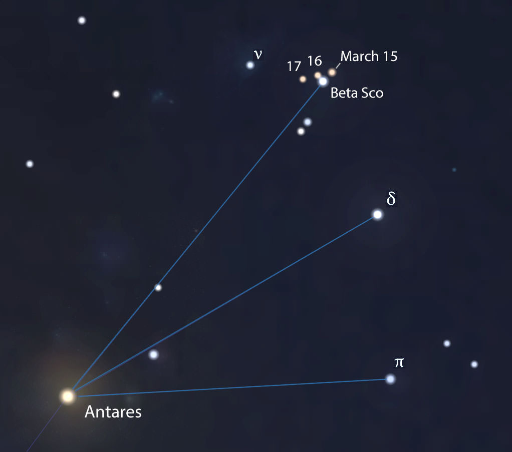
Face south tomorrow morning at the start of dawn and you might have to look twice for Beta Scorpii. Bright Mars stands right next to the star and will pass very close to the star on Wednesday morning, March 16. Diagram: Bob King, source: Stellarium
Planets can sneak up on you. Especially the ones that don’t rise till you’re in bed. Take Mars for instance. It’s been ambling east along the morning zodiac all winter long; today it enters Scorpius, rising around 1:30 a.m. Not two days later, the planet will have a spectacularly close conjunction with Beta Scorpii, the topmost star in the scorpion’s head.
This close up of the head of Scorpius shows Mars’ progress over the next three mornings. Positions are shown for 5:30 a.m. CDT. Diagram: Bob King, source: Stellarium
Also known as Graffias, Beta shines at magnitude +2.6 next to the fiery, zero-magnitude Mars. With their striking color contrast, the two would make a superb ring setting: a tiny diamond nestled next to a plump garnet. They’ll be together for several mornings, their separation changing each day: 15 arc minutes on Tuesday (1/2 the diameter of the Full Moon); 9 arc minutes when closest on Wednesday and back out to 23 minutes on Thursday.
In a telescope, diminutive Mars pairs up with gorgeous Graffias. North is up and left. Beta-1, the brighter of the two, has an additional 1oth magnitude companion half an arc-second away, while Beta-2 is also double with a faint companion 1/10th of arc second distant. That’s not all. Beta-1 is an exceedingly close binary — making Graffias at least a five-star system! Diagram: Bob King , source: Stellarium
It’s a gas to see two celestial objects approach so closely, but this conjunction offers a rare treat. Did you know that Beta is one of the finest double stars in the sky? It has a fifth magnitude companion 14 arc seconds northeast of the primary. Any telescope will split this jewel and show Mars in the same field of view at both high and low magnifications. That’s just so cool — I sure hope you’ll get to see them.
Mars, in gibbous phase, is still small but its larger surface features are now visible in modest-sized telescopes. This photo, taken on March 13th, shows Mare Acidalium in the planet’s northern hemisphere (top) and a hint of the north polar cap. Sinus Aurorae and Mare Erythraeum dominate the south. Click for a Mars map. Credit: Anthony Wesley
Mars now measures 10 arc seconds in diameter, small for sure, but big enough to see the larger dark markings and a hint of the north polar cap. The planet is heading for opposition on May 22nd, when it will shine at magnitude -2.0 (brighter than Sirius) with a disk 18.4 arc seconds across, its biggest and closest since 2005.
Let this week’s lovely conjunction serve as a warm-up to the forthcoming season of Mars.
Black-hole-powered galaxies called blazars are the most common sources detected by NASA's Fermi Gamma-ray Space Telescope. They are sources of neutrinos and cosmic rays.
Credits: M. Weiss/CfA
Way up in the constellation Cancer there’s a 14th magnitude speck of light you can claim in a 10-inch or larger telescope. If you saw it, you might sniff at something so insignificant, yet it represents the final farewell of chewed up stars as their remains whirl down the throat of an 18 billion solar mass black hole, one of the most massive known in the universe.
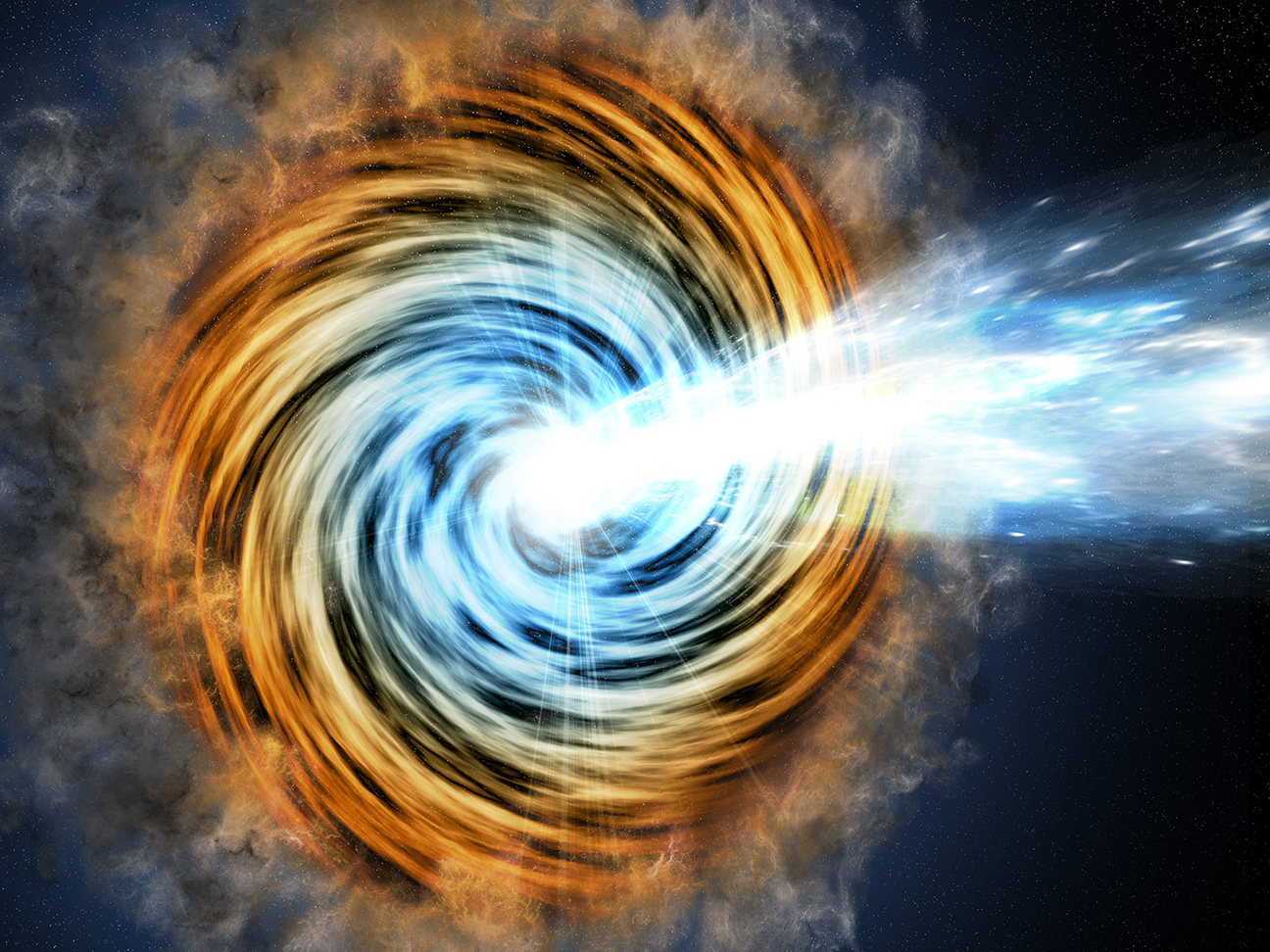
Artist’s view of a black hole-powered blazar (a type of quasar) lighting up the center of a remote galaxy. As matter falls toward the supermassive black hole at the galaxy’s center, some of it is accelerated outward at nearly the speed of light along jets pointed in opposite directions. When one of the jets happens to be aimed in the direction of Earth, as illustrated here, the galaxy appears especially bright and is classified as a blazar. Credits: M. Weiss/CfA
Astronomers know the object as OJ 287, a quasar that lies 3.5 billion light years from Earth. Quasars or quasi-stellar objects light up the centers of many remote galaxies. If we could pull up for a closer look, we’d see a brilliant, flattened accretion disk composed of heated star-stuff spinning about the central black hole at extreme speeds.
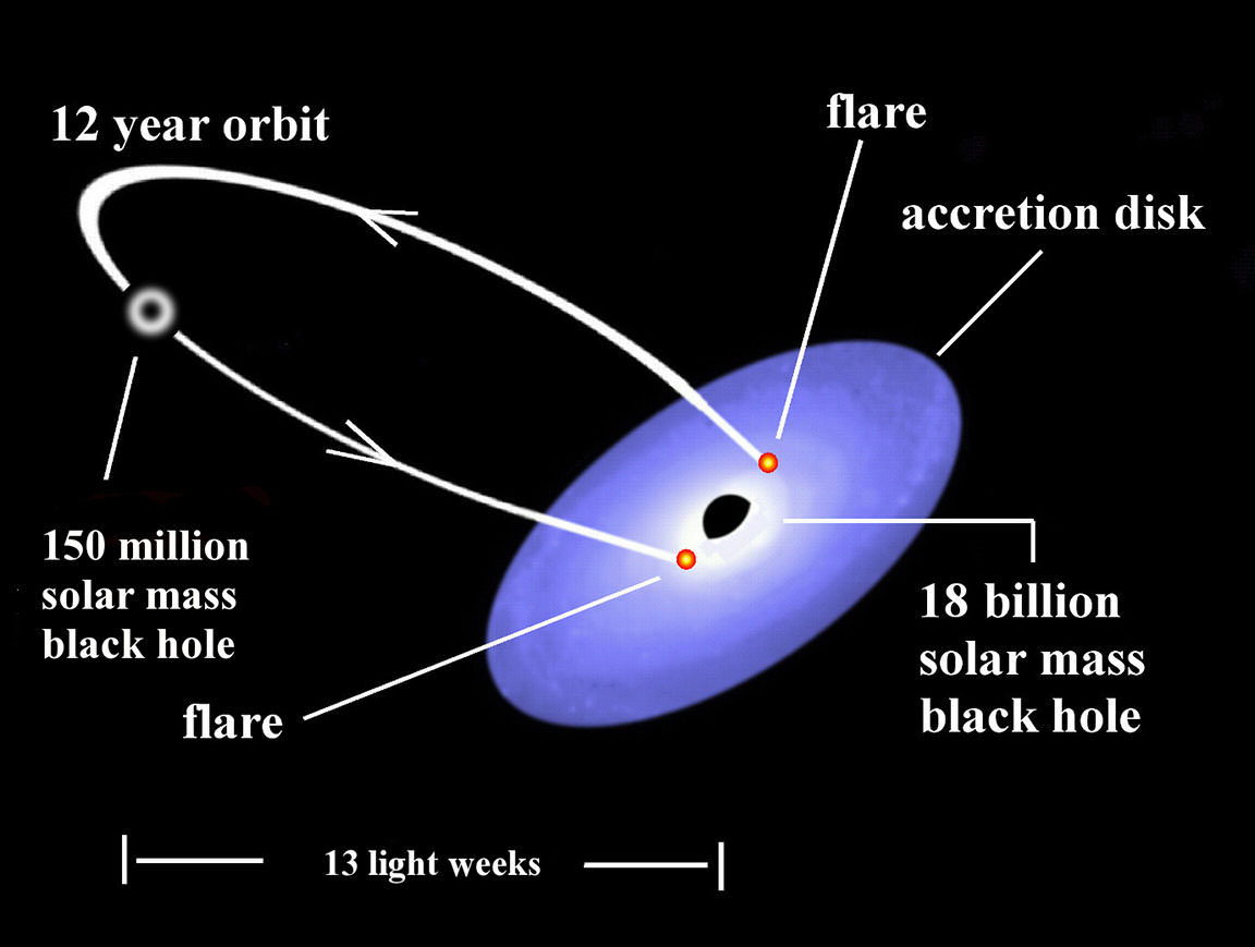
An illustration of the binary black hole system, OJ 287, showing the massive black hole surrounded by an accretion disk. A second, smaller black hole is believed to orbit the larger. When it intersects the larger’s disk coming and going, astronomers see a pair of bright flares. The predictions of the model are verified by observations. Credit: University of Turku
As matter gets sucked down the hole, jets of hot plasma and energetic light shoot out perpendicular to the disk. And if we’re so privileged that one of those jet happens to point directly at us, we call the quasar a “blazar”. Variability of the light streaming from the heart of a blazar is so constant, the object practically flickers.
Long exposures made with the Hubble Space Telescope showing brilliant quasars flaring in the hearts of six distant galaxies. Credit: NASA/ESA
A recent observational campaign involving more than two dozen optical telescopes and NASA’s space based SWIFT X-ray telescope allowed a team of astronomers to measure very accurately the rotational rate the black hole powering OJ 287 at one third the maximum spin rate — about 56,000 miles per second (90,000 kps) — allowed in General Relativity A careful analysis of these observations show that OJ 287 has produced close-to-periodic optical outbursts at intervals of approximately 12 years dating back to around 1891. A close inspection of newer data sets reveals the presence of double-peaks in these outbursts.
Illustration of a gradually precessing orbit similar to the precessing orbit of the smaller smaller black hole orbiting the larger in OJ 287. Credit: Willow W / Wikipedia
To explain the blazar’s behavior, Prof. Mauri Valtonen of the University of Turku (Finland) and colleagues developed a model that beautifully explains the data if the quasar OJ 287 harbors not one buy two unequal mass black holes — an 18 billion mass one orbited by a smaller black hole.
OJ 287 is visible due to the streaming of matter present in the accretion disk onto the largest black hole. The smaller black hole passes through the larger’s the accretion disk during its orbit, causing the disk material to briefly heat up to very high temperatures. This heated material flows out from both sides of the accretion disk and radiates strongly for weeks, causing the double peak in brightness.
The orbit of the smaller black hole also precesses similar to how Mercury’s orbit precesses. This changes when and where the smaller black hole passes through the accretion disk. After carefully observing eight outbursts of the black hole, the team was able to determine not only the black holes’ masses but also the precession rate of the orbit. Based on Valtonen’s model, the team predicted a flare in late November 2015, and it happened right on schedule.
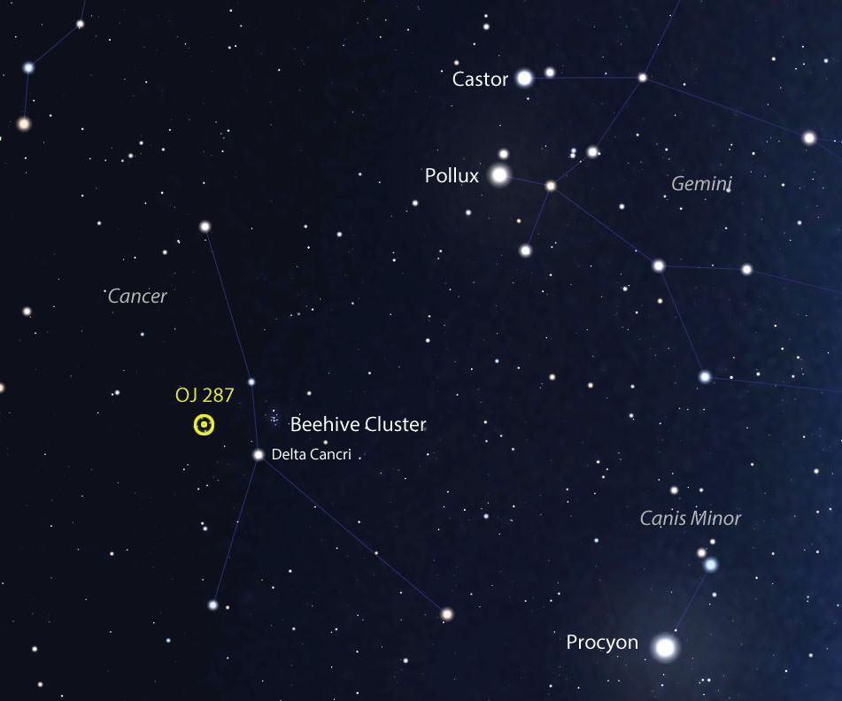
OJ 287 has been fluctuating around 13.5-140 magnitude lately. You can spot it in a 10-inch or larger scope in Cancer not far from the Beehive Cluster. Click the image for a detailed AAVSO finder chart. Diagram: Bob King, source: Stellarium
The timing of this bright outburst allowed Valtonen and his co-workers to directly measure the rotation rate of the more massive black hole to be nearly 1/3 the speed of light. I’ve checked around and as far as I can tell, this would make it the fastest spinning object we know of in the universe. Getting dizzy yet?
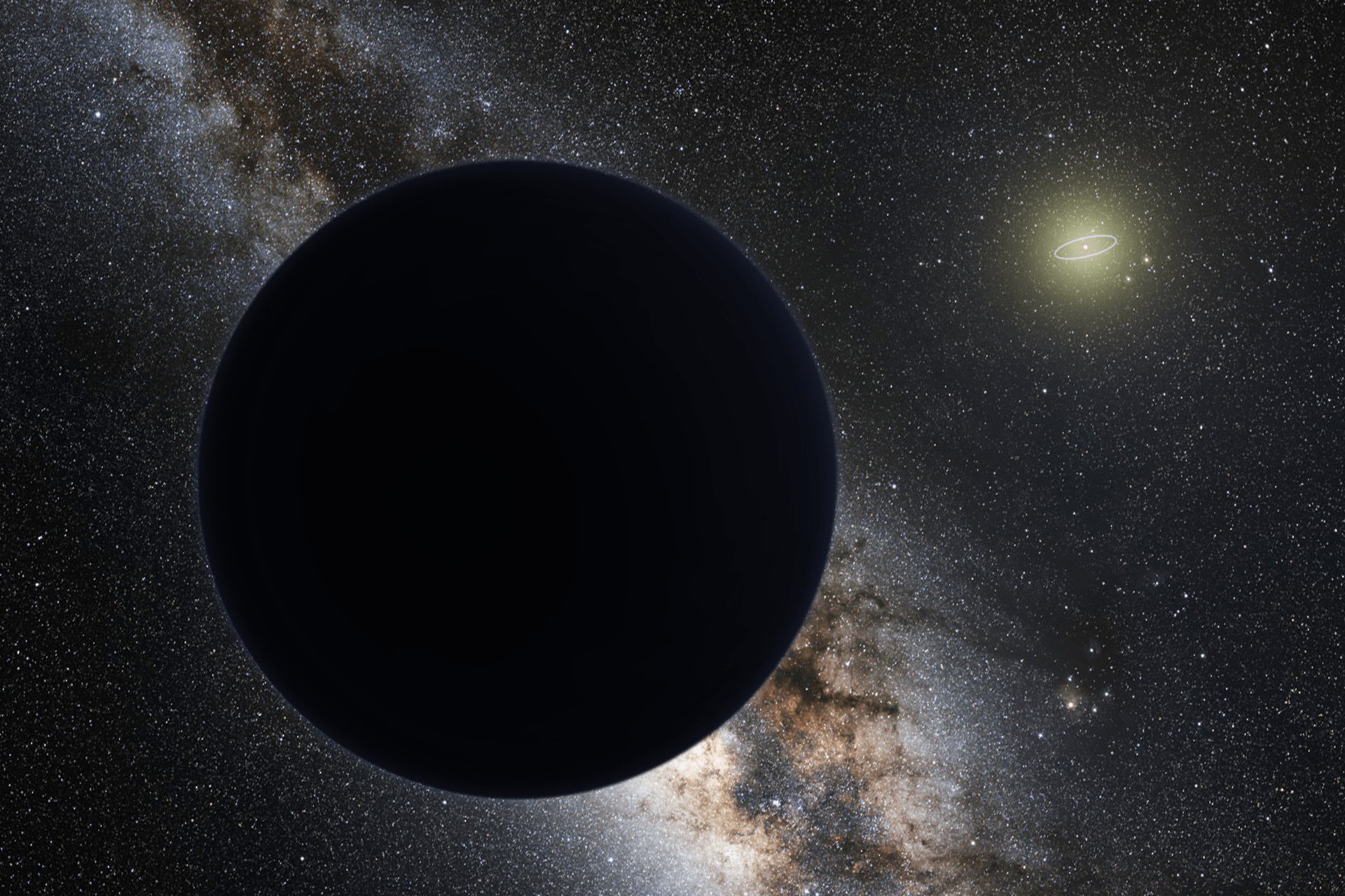
Artist's impression of Planet Nine, blocking out the Milky Way. The Sun is in the distance, with the orbit of Neptune shown as a ring. Credit: ESO/Tomruen/nagualdesign
On January 20th, 2016, researchers Konstantin Batygin and Michael E. Brown of Caltech announced that they had found evidence that hinted at the existence of a massive planet at the edge of the Solar System. Based on mathematical modeling and computer simulations, they predicted that this planet would be a super-Earth, two to four times Earth’s size and 10 times as massive. They also estimated that, given its distance and highly elliptical orbit, it would take 10,000 – 20,000 years to orbit the Sun.
Since that time, many researchers have responded with their own studies about the possible existence of this mysterious “Planet 9”. One of the latest comes from the University of Arizona, where a research team from the Lunar and Planetary Laboratory have indicated that the extreme eccentricity of distant Kuiper Belt Objects (KBOs) might indicate that they crossed paths with a massive planet in the past.
For some time now, it has been understood that there are a few known KBOs who’s dynamics are different than those of other belt objects. Whereas most are significantly controlled by the gravity of the gas giants planets in their current orbits (particularly Neptune), certain members of the scattered disk population of the Kuiper Belt have unusually closely-spaced orbits.
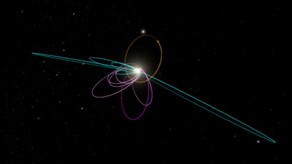
The orbits of Neptune (magenta), Sedna (dark magenta), a series of Kuiper belt objects (cyan), and the hypothetical Planet 9 (orange). Credit: Caltech/R. Hurt (IPAC)
When Batygin and Brown first announced their findings back in January, they indicated that these objects instead appeared to be highly clustered with respect to their perihelion positions and orbital planes. What’s more, their calculation showed that the odds of this being a chance occurrence were extremely low (they calculated a probability of 0.007%).
Instead, they theorized that it was a distant eccentric planet that was responsible for maintaining the orbits of these KBOs. In order to do this, the planet in question would have to be over ten times as massive as Earth, and have an orbit that lay roughly on the same plane (but with a perihelion oriented 180° away from those of the KBOs).
Such a planet not only offered an explanation for the presence of high-perihelion Sedna-like objects – i.e. planetoids that have extremely eccentric orbits around the Sun. It would also help to explain where distant and highly inclined objects in the outer Solar System come from, since their origins have been unclear up until this point.
In a paper titled “Coralling a distant planet with extreme resonant Kuiper belt objects“, the University of Arizona research team – which included Professor Renu Malhotra, Dr. Kathryn Volk, and Xianyu Wang – looked at things from another angle. If in fact Planet 9 were crossing paths with certain high-eccentricity KBOs, they reasoned, it was a good bet that its orbit was in resonance with these objects.
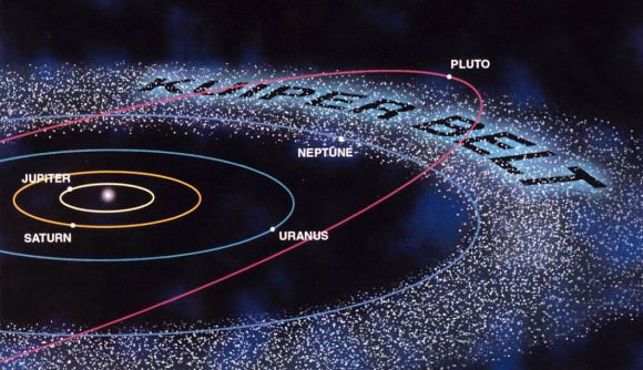
Pluto and its cohorts in the icy-asteroid-rich Kuiper Belt beyond the orbit of Neptune. Credit: NASA
To break it down, small bodies are ejected from the Solar System all the time due to encounters with larger objects that perturb their orbits. In order to avoid being ejected, smaller bodies need to be protected by orbital resonances. While the smaller and larger objects may pass within each others’ orbital path, they are never close enough that they would able to exert a significant influence on each other.
This is how Pluto has remained a part of the Solar System, despite having an eccentric orbit that periodically cross Neptune’s path. Though Neptune and Pluto cross each others orbit, they are never close enough to each other that Neptune’s influence would force Pluto out of our Solar System. Using this same reasoning, they hypothesized that the KBOs examined by Batygin and Brown might be in an orbital resonance with the Planet 9.
As Dr. Malhotra, Volk and Wang told Universe Today via email:
“The extreme Kuiper belt objects we investigate in our paper are distinct from the others because they all have very distant, very elliptical orbits, but their closest approach to the Sun isn’t really close enough for them to meaningfully interact with Neptune. So we have these six observed objects whose orbits are currently fairly unaffected by the known planets in our Solar System. But if there’s another, as yet unobserved planet located a few hundred AU from the Sun, these six objects would be affected by that planet.”
After examining the orbital periods of these six KBOs – Sedna, 2010 GB174, 2004 VN112, 2012 VP113, and 2013 GP136 – they concluded that a hypothetical planet with an orbital period of about 17,117 years (or a semimajor axis of about 665 AU), would have the necessary period ratios with these four objects. This would fall within the parameters estimated by Batygin and Brown for the planet’s orbital period (10,000 – 20,000 years).
Animated diagram showing the spacing of the Solar Systems planet’s, the unusually closely spaced orbits of six of the most distant KBOs, and the possible “Planet 9”. Credit: Caltech/nagualdesign
Their analysis also offered suggestions as to what kind of resonance the planet has with the KBOs in question. Whereas Sedna’s orbital period would have a 3:2 resonance with the planet, 2010 GB174 would be in a 5:2 resonance, 2994 VN112 in a 3:1, 2004 VP113 in 4:1, and 2013 GP136 in 9:1. These sort of resonances are simply not likely without the presence of a larger planet.
“For a resonance to be dynamically meaningful in the outer Solar System, you need one of the objects to have enough mass to have a reasonably strong gravitational effect on the other,” said the research team. “The extreme Kuiper belt objects aren’t really massive enough to be in resonances with each other, but the fact that their orbital periods fall along simple ratios might mean that they each are in resonance with a massive, unseen object.”
But what is perhaps most exciting is that their findings could help to narrow the range of Planet 9’s possible location. Since each orbital resonance provides a geometric relationship between the bodies involved, the resonant configurations of these KBOs can help point astronomers to the right spot in our Solar System to find it.
But of course, Malhotra and her colleagues freely admit that several unknowns remain, and further observation and study is necessary before Planet 9 can be confirmed:
“There are a lot of uncertainties here. The orbits of these extreme Kuiper belt objects are not very well known because they move very slowly on the sky and we’ve only observed very small portions of their orbital motion. So their orbital periods might differ from the current estimates, which could make some of them not resonant with the hypothetical planet. It could also just be chance that the orbital periods of the objects are related; we haven’t observed very many of these types of objects, so we have a limited set of data to work with.”
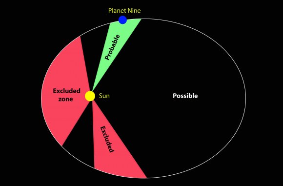
Estimates of Planet Nine’s “possible” and “probable” zones. by French scientists based on a careful study of Saturn’s orbit and using mathematical models. Source: CNRS, Cote d’Azur and Paris observatories. Credit: Bob King
Ultimately, astronomers and the rest of us will simply have to wait on further observations and calculations. But in the meantime, I think we can all agree that the possibility of a 9th Planet is certainly an intriguing one! For those who grew up thinking that the Solar System had nine planets, these past few years (where Pluto was demoted and that number fell to eight) have been hard to swallow.
But with the possible confirmation of this Super-Earth at the outer edge of the Solar System, that number could be pushed back up to nine soon enough!
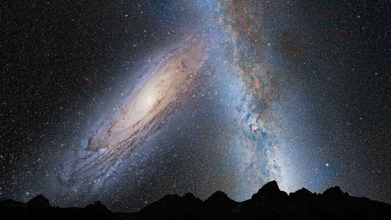
Artist's illustration of the Andromeda galaxy and the Milky Way, the two largest galaxies in the Local Group. Credit: NASA
In about 4 billion years, scientists estimate that the Andromeda and the Milky Way galaxies are expected to collide, based on data from the Hubble Space Telescope. And when they merge, they will give rise to a super-galaxy that some are already calling Milkomeda or Milkdromeda (I know, awful isn’t it?) While this may sound like a cataclysmic event, these sorts of galactic collisions are quite common on a cosmic timescale.
As an international group of researchers from Japan and California have found, galactic “hookups” were quite common during the early universe. Using data from the Hubble Space Telescope and the Subaru Telescope at in Mauna Kea, Hawaii, they have discovered that 1.2 billion years after the Big Bang, galactic clumps grew to become large galaxies by merging. As part of the Hubble Space Telescope (HST) “Cosmic Evolution Survey (COSMOS)”, this information could tell us a great about the formation of the early universe.
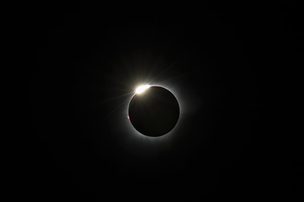
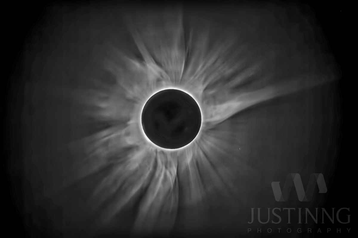
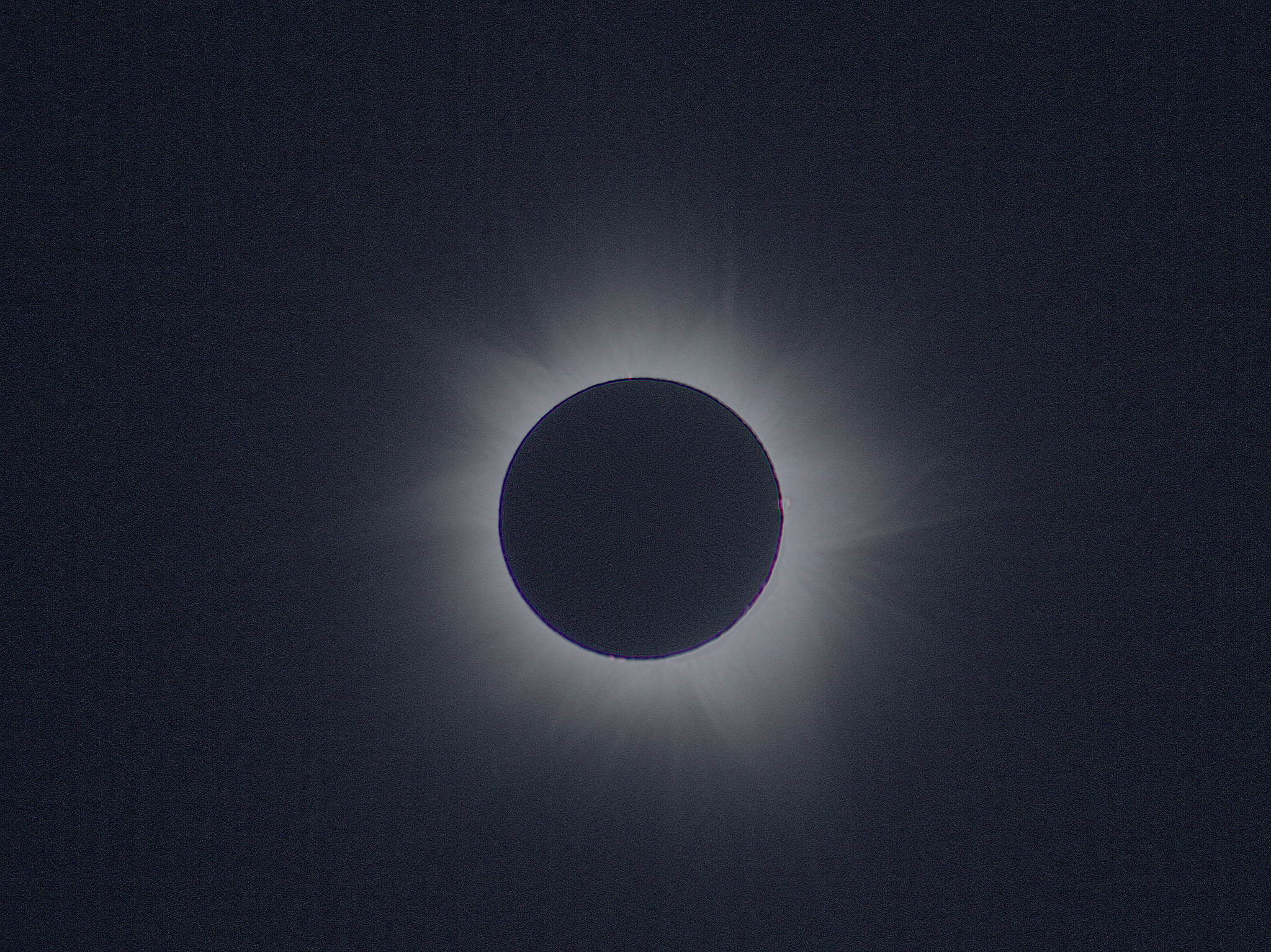
Totality! A fine capture featuring the 'diamond ring' effect as sunlight streams through lunar valleys. Image credit and copyright: Justin Ng Astrophotography
The Moon’s shadow kissed the Earth earlier today, providing a fine show from southeast Asia, to the southern shores of Alaska. We wrote about the only total solar eclipse for 2016 yesterday. This is it, the last total solar eclipse prior to the return of totality for the contiguous United States on August 21st, 2017.
Cloud cover over the region was a toss up, with clear skies for some, and cloudy skies for others. Those towards the western end of the track where the eclipsed rising Sun sat low on the horizon seemed to have fared worst.
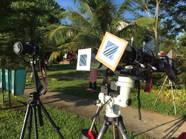
Clouds thwarted a Malaysian team that had journeyed to Indonesia to view the eclipse (including Sharin Ahmad @shahgazer), though they were at the ready. Image credit and copyright: Sharin Ahmad.
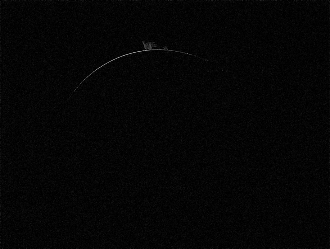
Update: Sometimes, the camera sees what the eye misses. The Malaysian team did indeed manage to nab a fine display of Bailey’s Beads in the moments leading up to totality through a thin gap in the clouds:
Sunlight, interupted. A welcome photobomb courtesy of the Earth’s Moon. Image credit and copyright: Shahrin Ahmad. (@shahgazer)
Skies dawned clear to the east over the Indonesian islands on the morning of the eclipse, and the joint NASA/Exploratorium webcast from the remote atoll of Woleai in Micronesia was a success.
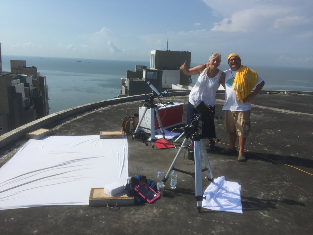
A ‘helipad solar observatory’ readied for the eclipse. Image credit and copyright: Patrick Poitevin.
Observing from a helipad Balikpanpan, Indonesia, veteran eclipse chaser Patrick Poitevin said: “What an eclipse! Vertically clear sky throughout the entire eclipse from our ‘private’ helipad in Balikpapan. Only slight haze now and then. Asymmetric corona, with bright and prominent snow white streamer. Venus, Mercury easily visible long before, and shadow bands post totality. Fabulous! All so pretty!!! Marked the second Saros 130 for Jo and the 3rd for me.”
Many viewers noted a fine solar prominence on the solar limb seen during totality. Patrick Poitevin caught the prominence using a hydrogen-alpha solar telescope just moments before the onset of totality. Image credit: Patrick Poitevin.
Indeed, catching a ‘triple saros’ known as an exeligmos is a noteworthy lifetime accomplishment.
09 March 2016 – Total Solar Eclipse from Palu, Indonesia. Image credit and copyright: Justin Ng.
Many witnessed the eclipse via Slooh’s live webcast from the path of totality, which is now archived in its entirety on YouTube.
Totality, as witnessed by the Slooh team in Indonesia. Image credit: www.slooh.com
As of writing this, no views from space have surfaced, though we suspect this will change as the day goes on. Word is that the Alaskan Airlines flight that modified their flight plan to catch the eclipse was successful as well. Check back, as we’ll be dropping in more images as they trickle in from the field throughout the day.
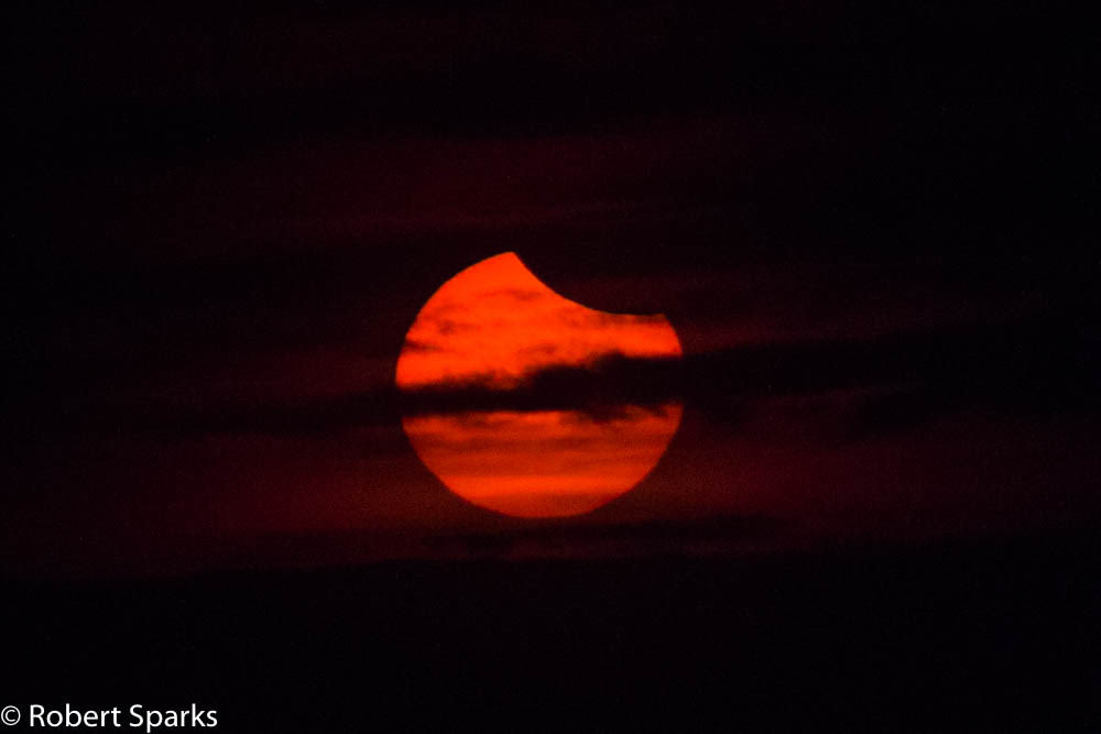
The partial phases of today’s eclipse as seen from Lava Lava, Hawaii. Image credit and copyright: Rob Sparks (@halfastro)
Update: Scratch that… Japan’s Himawari-8 weather satellite did indeed nab views of the umbra of the Moon as it raced across the Pacific:
An animation of today’s total solar eclipse as seen from space. Image credit: The Meteorological Satellite Center of JAMA.
Though the eclipse was almost entirely over water after the umbra departed SE Asia, regions around the path were treated to a fine partial eclipse, including residents of Hawaii:
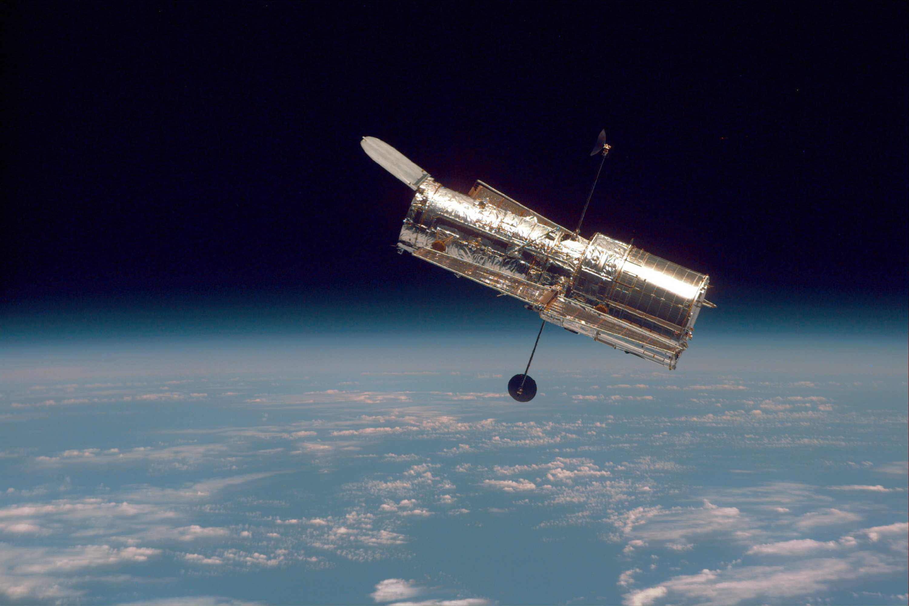
China has plans to build a new space telescope which should outperform Hubble. According to the Chinese English Language Daily, the new telescope will be similar to Hubble, but will have a field of view that is 300 times larger. The new telescope, which has not been named yet, will have the ability to dock with China’s modular space station, the Tiangong.
The China National Space Administration has come up with a solution to a problem that dogged the Hubble Telescope. Whenever the Hubble needed repairs or maintenance, a shuttle mission had to be planned so astronauts could service it. China will avoid this problem with its innovative solution. The Chinese telescope will keep its distance from the Tiangong, but if repairs or maintenance are needed, it can dock with Tiangong.
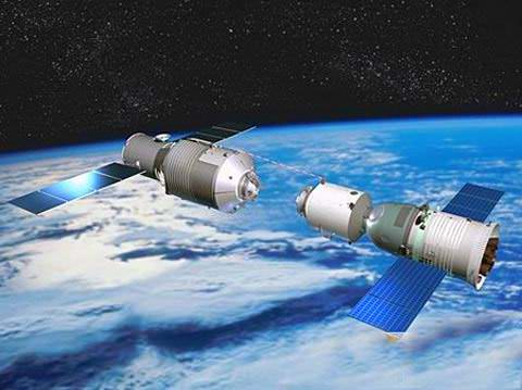
No date has been given for the launch of this new telescope, but its plans must be intertwined with plans for the modular Tiangong space station. Tiangong-1 was launched in 2011 and has served as a crewed laboratory and a technological test-bed. The Tiangong-2, which has room for a crew of 3 and life support for twenty days, is expected to be launched sometime in 2016. The Tiangong-3 will provide life support for 3 people for 40 days and will expand China’s capabilities in space. It’s not expected to launch until sometime in the 2020’s, so the space telescope will likely follow its launch.
An artist’s rendering of the Tiangong-1 module, China’s space station, which was launched to space in September, 2011. To the right is a Shenzhou spacecraft, preparing to dock with the module. Image Credit: CNSA
The telescope, according to the People’s Daily Online, will take 10 years to capture images of 40% of space, with a precision equal to Hubble’s. China hopes this data will allow it to make breakthroughs in the understanding of the origin, development, and evolution of the universe.
This all sounds great, but there’s a shortage of facts. When other countries and space agencies announce projects like this, they give dates and timelines, and details about the types of cameras and sensors. They talk about exactly what it is they plan to study and what results they hope to achieve. It’s difficult to say what level of detail has gone into the planning for this space telescope. It’s also difficult to say how the ‘scope will dock with the space station.
It may be that China is nervous about spying and doesn’t want to reveal any technical detail. Or it may be that China likes announcing things that make it look technologically advanced. (China is in a space race with India, and likes to boast of its prowess.) In any case, they’ve been talking about a space telescope for many years now. But a little more information would be nice.
Come on China. Give us more info. We’re not spies. We promise.
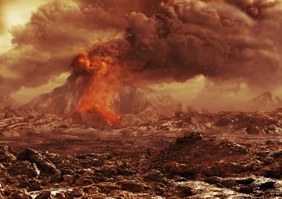
Artist's impression of the surface of Venus. Credit: ESA/AOES
Continuing with our “Definitive Guide to Terraforming“, Universe Today is happy to present to our guide to terraforming Venus. It might be possible to do this someday, when our technology advances far enough. But the challenges are numerous and quite specific.
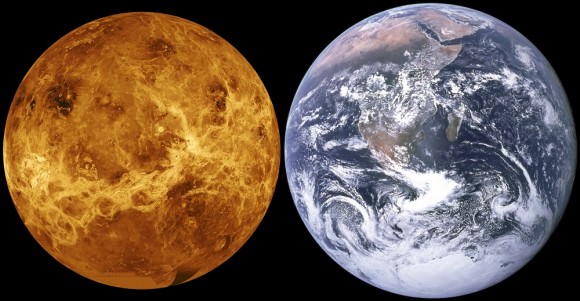
The planet Venus is often referred to as Earth’s “Sister Planet”, and rightly so. In addition to being almost the same size, Venus and Earth are similar in mass and have very similar compositions (both being terrestrial planets). As a neighboring planet to Earth, Venus also orbits the Sun within its “Goldilocks Zone” (aka. habitable zone). But of course, there are many key difference between the planets that make Venus uninhabitable.
For starters, it’s atmosphere over 90 times thicker than Earth’s, its average surface temperature is hot enough to melt lead, and the air is a toxic fume consisting of carbon dioxide and sulfuric acid. As such, if humans want to live there, some serious ecological engineering – aka. terraforming – is needed first. And given its similarities to Earth, many scientists think Venus would be a prime candidate for terraforming, even more so than Mars!
Over the past century, the concept of terraforming Venus has appeared multiple times, both in terms of science fiction and as the subject of scholarly study. Whereas treatments of the subject were largely fantastical in the early 20th century, a transition occurred with the beginning of the Space Age. As our knowledge of Venus improved, so too did the proposals for altering the landscape to be more suitable for human habitation.
Venus is also considered a prime candidate for terraforming. Credit: NASA/JPL/io9.com
Examples in Fiction:
Since the early 20th century, the idea of ecologically transforming Venus has been explored in fiction. The earliest known example is Olaf Stapleton’sLast And First Men(1930), two chapters of which are dedicated to describing how humanity’s descendants terraform Venus after Earth becomes uninhabitable; and in the process, commit genocide against the native aquatic life.
By the 1950s and 60s, owing to the beginning of the Space Age, terraforming began to appear in many works of science fiction. Poul Anderson also wrote extensively about terraforming in the 1950s. In his 1954 novel, The Big Rain, Venus is altered through planetary engineering techniques over a very long period of time. The book was so influential that the term term “Big Rain” has since come to be synonymous with the terraforming of Venus.
In 1991, author G. David Nordley suggested in his short story (“The Snows of Venus”) that Venus might be spun-up to a day-length of 30 Earth days by exporting its atmosphere of Venus via mass drivers. Author Kim Stanley Robinson became famous for his realistic depiction of terraforming in the Mars Trilogy – which included Red Mars, Green Mars and Blue Mars.
In 2012, he followed this series up with the release of 2312, a science fiction novel that dealt with the colonization of the entire Solar System – which includes Venus. The novel also explored the many ways in which Venus could be terraformed, ranging from global cooling to carbon sequestration, all of which were based on scholarly studies and proposals.
Artist’s conception of a terraformed Venus, showing a surface largely covered in oceans. Credit: Wikipedia Commons/Ittiz
Proposed Methods:
The first proposed method of terraforming Venus was made in 1961 by Carl Sagan. In a paper titled “The Planet Venus“, he argued for the use of genetically engineered bacteria to transform the carbon in the atmosphere into organic molecules. However, this was rendered impractical due to the subsequent discovery of sulfuric acid in Venus’ clouds and the effects of solar wind.
In his 1991 study “Terraforming Venus Quickly“, British scientist Paul Birch proposed bombarding Venus’ atmosphere with hydrogen. The resulting reaction would produce graphite and water, the latter of which would fall to the surface and cover roughly 80% of the surface in oceans. Given the amount of hydrogen needed, it would have to harvested directly from one of the gas giant’s or their moon’s ice.
The proposal would also require iron aerosol to be added to the atmosphere, which could be derived from a number of sources (i.e. the Moon, asteroids, Mercury). The remaining atmosphere, estimated to be around 3 bars (three times that of Earth), would mainly be composed of nitrogen, some of which will dissolve into the new oceans, reducing atmospheric pressure further.
Another idea is to bombard Venus with refined magnesium and calcium, which would sequester carbon in the form of calcium and magnesium carbonates. In their 1996 paper, “The stability of climate on Venus“, Mark Bullock and David H. Grinspoon of the University of Colorado at Boulder indicated that Venus’ own deposits of calcium and magnesium oxides could be used for this process. Through mining, these minerals could be exposed to the surface, thus acting as carbon sinks.
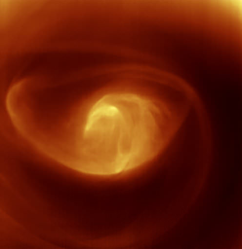
A mass of swirling gas and cloud at Venus’ south pole. Credit: ESA/VIRTIS/INAF-IASF/Obs. de Paris-LESIA/Univ. Oxford.
However, Bullock and Grinspoon also claim this would have a limited cooling effect – to about 400 K (126.85 °C; 260.33 °F) and would only reduce the atmospheric pressure to an estimated 43 bars. Hence, additional supplies of calcium and magnesium would be needed to achieve the 8×10²⁰ kg of calcium or 5×10²⁰ kg of magnesium required, which would most likely have to be mined from asteroids.
The concept of solar shades has also been explored, which would involve using either a series of small spacecraft or a single large lens to divert sunlight from a planet’s surface, thus reducing global temperatures. For Venus, which absorbs twice as much sunlight as Earth, solar radiation is believed to have played a major role in the runaway greenhouse effect that has made it what it is today.
Such a shade could be space-based, located in the Sun–Venus L1 Lagrangian point, where it would prevent some sunlight from reaching Venus. In addition, this shade would also serve to block the solar wind, thus reducing the amount of radiation Venus’ surface is exposed to (another key issue when it comes to habitability). This cooling would result in the liquefaction or freezing of atmospheric CO², which would then be depsotied on the surface as dry ice (which could be shipped off-world or sequestered underground).
Alternately, solar reflectors could be placed in the atmosphere or on the surface. This could consist of large reflective balloons, sheets of carbon nanotubes or graphene, or low-albedo material. The former possibility offers two advantages: for one, atmospheric reflectors could be built in-situ, using locally-sourced carbon. Second, Venus’ atmosphere is dense enough that such structures could easily float atop the clouds.
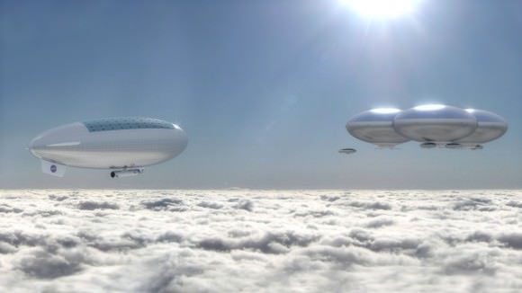
Artist’s concept of a Venus cloud city – part of NASA’s High Altitude Venus Operational Concept (HAVOC) plan. Credit: Advanced Concepts Lab/NASA Langley Research Center
NASA scientist Geoffrey A. Landis has also proposed that cities could be built above Venus’ clouds, which in turn could act as both a solar shield and as processing stations. These would provide initial living spaces for colonists, and would act as terraformers, gradually converting Venus’ atmosphere into something livable so the colonists could migrate to the surface.
Another suggestion has to do with Venus’ rotational speed. Venus rotates once every 243 days, which is by far the slowest rotation period of any of the major planets. As such, Venus’s experiences extremely long days and nights, which could prove difficult for most known Earth species of plants and animals to adapt to. The slow rotation also probably accounts for the lack of a significant magnetic field.
To address this, British Interplanetary Society member Paul Birch suggested creating a system of orbital solar mirrors near the L1 Lagrange point between Venus and the Sun. Combined with a soletta mirror in polar orbit, these would provide a 24-hour light cycle.
It has also been suggested that Venus’ rotational velocity could be spun-up by either striking the surface with impactors or conducting close fly-bys using bodies larger than 96.5 km (60 miles) in diameter. There is also the suggestion of using using mass drivers and dynamic compression members to generate the rotational force needed to speed Venus up to the point where it experienced a day-night cycle identical to Earth’s (see above).
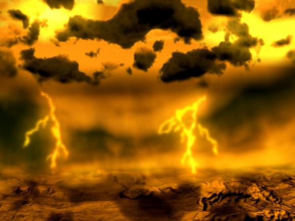
Artist’s impression of Venus’ thick atmosphere, complete with lighting strikes and sulfuric acid rains. Credit: ESA
Then there’s the possibility of removing some of Venus’ atmosphere, which could accomplished in a number of ways. For starters, impactors directed at the surface would blow some of the atmosphere off into space. Other methods include space elevators and mass accelerators (ideally placed on balloons or platforms above the clouds), which could gradually scoop gas from the atmosphere and eject it into space.
Potential Benefits:
One of the main reasons for colonizing Venus, and altering its climate for human settlement, is the prospect of creating a “backup location” for humanity. And given the range of choices – Mars, the Moon, and the Outer Solar System – Venus has several things going for it the others do not. All of these highlight why Venus is known as Earth’s “Sister Planet”.
For starters, Venus is a terrestrial planet that is similar in size, mass and composition to Earth. This is why Venus has similar gravity to Earth, which is about of what we experience 90% (or 0.904 g, to be exact. As a result, humans living on Venus would be at a far lower risk of developing health problems associated with time spent in weightlessness and microgravity environments – such as osteoporosis and muscle degeneration.
Venus’s relative proximity to Earth would also make transportation and communications easier than with most other locations in the solar system. With current propulsion systems, launch windows to Venus occur every 584 days, compared to the 780 days for Mars. Flight time is also somewhat shorter since Venus is the closest planet to Earth. At it’s closest approach, it is 40 million km distant, compared to 55 million km for Mars.
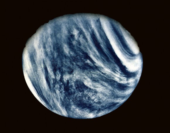
On Feb. 5, 1974, NASA’s Mariner 10 mission took this first close-up photo of Venus during 1st gravity assist flyby. Credit: NASA
Another reason has to do with Venus’ runaway greenhouse effect, which is the reason for the planet’s extreme heat and atmospheric density. In testing out various ecological engineering techniques, our scientists would learn a great deal about their effectiveness. This information, in turn, will come in mighty handy in the ongoing fight against Climate Change here on Earth.
And in the coming decades, this fight is likely to become rather intense. As the NOAA reported in March of 2015, carbon dioxide levels in the atmosphere have now surpassed 400 ppm, a level not seen since the the Pliocene Era – when global temperatures and sea level were significantly higher. And as a series of scenarios computed by NASA show, this trend is likely to continue until 2100, with severe consequences.
In one scenario, carbon dioxide emissions will level off at about 550 ppm toward the end of the century, resulting in an average temperature increase of 2.5 °C (4.5 °F). In the second scenario, carbon dioxide emissions rise to about 800 ppm, resulting in an average increase of about 4.5 °C (8 °F). Whereas the increases predicted in the first scenario are sustainable, in the latter scenario, life will become untenable on many parts of the planet.
So in addition to creating a second home for humanity, terraforming Venus could also help to ensure that Earth remains a viable home for our species. And of course, the fact that Venus is a terrestrial planet means that it has abundant natural resources that could be harvested, helping humanity to achieve a “post-scarcity” economy.
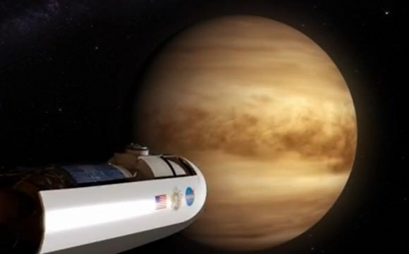
Artist’s concept of the High Altitude Venus Operational Concept (HAVOC) mission approaching the planet. Credit: NASA Langley Research Center/YouTube.
Challenges:
Beyond the similarities Venus’ has with Earth (i.e. size, mass and composition), there are numerous differences that would make terraforming and colonizing it a major challenge. For one, reducing the heat and pressure of Venus’ atmosphere would require a tremendous amount of energy and resources. It would also require infrastructure that does not yet exist and would be very expensive to build.
For instance, it would require immense amounts of metal and advanced materials to build an orbital shade large enough to cool Venus’ atmosphere to the point that its greenhouse effect would be arrested. Such a structure, if positioned at L1, would also need to be four times the diameter of Venus itself. It would have to be assembled in space, which would require a massive fleet of robot assemblers.
In contrast, increasing the speed of Venus’s rotation would require tremendous energy, not to mention a significant number of impactors that would have to cone from the outer solar System – mainly from the Kuiper Belt. In all of these cases, a large fleet of spaceships would be needed to haul the necessary material, and they would need to be equipped with advanced drive systems that could make the trip in a reasonable amount of time.
Currently, no such drive systems exist, and conventional methods – ranging from ion engines to chemical propellants – are neither fast or economical enough. To illustrate, NASA’s New Horizons mission took more than 11 years to get make its historic rendezvous with Pluto in the Kuiper Belt, using conventional rockets and the gravity-assist method.
Artist’s impression of the surface of Venus. Credit: ESA/AOES
Meanwhile, the Dawn mission, which relied relied on ionic propulsion, took almost four years to reach Vesta in the Asteroid Belt. Neither method is practical for making repeated trips to the Kuiper Belt and hauling back icy comets and asteroids, and humanity has nowhere near the number of ships we would need to do this.
The same problem of resources holds true for the concept of placing solar reflectors above the clouds. The amount of material would have to be large and would have to remain in place long after the atmosphere had been modified, since Venus’s surface is currently completely enshrouded by clouds. Also, Venus already has highly reflective clouds, so any approach would have to significantly surpass its current albedo (0.65) to make a difference.
And when it comes to removing Venus’ atmosphere, things are equally challenging. In 1994, James B. Pollack and Carl Sagan conducted calculations that indicated that an impactor measuring 700 km in diameter striking Venus at high velocity would less than a thousandth of the total atmosphere. What’s more, there would be diminishing returns as the atmosphere’s density decreases, which means thousands of giant impactors would be needed.
In addition, most of the ejected atmosphere would go into solar orbit near Venus, and – without further intervention – could be captured by Venus’s gravitational field and become part of the atmosphere once again. Removing atmospheric gas using space elevators would be difficult because the planet’s geostationary orbit lies an impractical distance above the surface, where removing using mass accelerators would be time-consuming and very expensive.
Size comparison of Venus and Earth. Credit: NASA/JPL/Magellan
Conclusion:
In sum, the potential benefits of terraforming Venus are clear. Humanity would have a second home, we would be able to add its resources to our own, and we would learn valuable techniques that could help prevent cataclysmic change here on Earth. However, getting to the point where those benefits could be realized is the hard part.
Like most proposed terraforming ventures, many obstacles need to be addressed beforehand. Foremost among these are transportation and logistics, mobilizing a massive fleet of robot workers and hauling craft to harness the necessary resources. After that, a multi-generational commitment would need to be made, providing financial resources to see the job through to completion. Not an easy task under the most ideal of conditions.
Suffice it to say, this is something that humanity cannot do in the short-run. However, looking to the future, the idea of Venus becoming our “Sister Planet” in every way imaginable – with oceans, arable land, wildlife and cities – certainly seems like a beautiful and feasible goal. The only question is, how long will we have to wait?
And if you liked the video posted above, come check out our Patreon page and find out how you can get these videos early while helping us bring you more great content!
Totality! The total solar eclipse of November 14th, 2012. Image credit: Narayan Mukkavilli
Ready for the ultimate in astronomical events? On the morning of Wednesday, March 9th, the Moon eclipses the Sun for viewers across southeast Asia.
Many intrepid umbraphiles are already in position for the spectacle. The event is the only total solar eclipse of 2016, and the penultimate total solar eclipse prior the ‘Big One’ crossing the continental United States on August 21st, 2017.
The path of tomorrow’s eclipse. Image credit: Great American Eclipse/Michael Zeiler
Tales of the Saros
This particular eclipse is member 52 of 73 eclipses in saros cycle 130, which runs from 1096 AD to 2394. If you saw the total solar eclipse which crossed South America on February 26th, 1998, then you caught the last solar eclipse from the same cycle.
An animation of the event. Image credit: NASA/GSFC/A.T. Sinclair
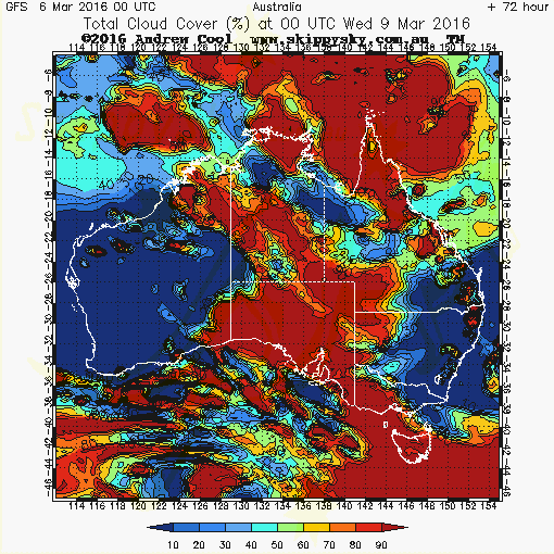
Weather prospects are dicey along the eclipse track, as March is typically the middle of monsoon season for southeast Asia. Most eclipse chasers have headed to the islands of Indonesia or cruises based nearby to witness the event. The point of greatest eclipse lies off of the southeastern coast of the Philippine Islands in the South China Sea, with a duration of 4 minutes and 10 seconds. Most observers, however, will experience a substantially shorter period of totality. For example, totality lasts only 2 minutes and 35 seconds over island of Ternate, where many eclipse chasers have gathered. The Sun will be 48 degrees above the horizon from the island during totality.
A great place to check cloud cover and weather prospects along the eclipse track is the Eclipsophile website.
A dicey sky: prospects for cloud cover over Australia. Image credit; SkippySky
The umbra of the Earth’s Moon will sweep across Sumatra at sunrise and across the island of Borneo, to landfall one last time for Indonesia over the island of North Maluku before sweeping across the central Pacific. This eclipse is unusual in that it makes landfall over a very few countries: the island nation of Indonesia, and just a few scattered atolls in Palau and Micronesia.
Partial phases of the eclipse are also visible from India at sunrise, across northeast Asia along the northernmost track, to central Australia in the south, and finally, to southern Alaskan coast at sunset. Honolulu Hawaii sees a 65% partial solar eclipse in the late afternoon on March 8th.
Expect great views, both from Earth and from space. We typically get images from solar observing spacecraft, to include the joint NASA/JAXA Hinode mission, and the European Space Agency’s PROBA-2 spacecraft. Both are in low-Earth orbit, and see a given eclipse as a swift, fleeting event. Other solar observatories—such as the Solar Heliospheric Observatory and the Solar Dynamics Observatory—occupy a different vantage point in space, and miss the eclipse.
The orientation of the Sun and planets at totality (click to enlarge). Image credit: Starry Night Education Software
As of this writing, we know of several folks that have made the journey to stand in the path of totality, to include Sharin Ahmad (@Shagazer), Michael Zeiler (@GreatAmericanEclipse) and Justin Ng.
Good luck and clear skies to all observers out there, awaiting darkness in the path of totality.
Live in the wrong hemisphere? There are several live webcasts planned from the eclipse zone:
NASA and the National Science Foundation are working with a team from San Francisco’s Exploratorium to bring a live webcast of the eclipse from the remote atoll island of Woleai, Micronesia. The feed starts at 7:00 EST/0:00 Universal Time (UT) and runs for just over three hours. You can follow the exploits of the team leading up to show time here.
The venerable Slooh will also feature a webcast of the eclipse with astronomer Paul Cox from Indonesia running for three hours starting at 6:00 PM EST/23:00 UT.
A view of the partial phases of the eclipse from the Hong Kong science center also starts at 5:30 PM EST/22:30 UT:
Don’t forget: though the eclipse occurs on the morning of March 9th local time in southeast Asia, the path crosses the International Dateline, and the webcasts kick off on the evening of Tuesday March 8th for North America.
And hey, Alaska Airlines flight 870 from Anchorage to Honolulu will divert from its flight plan slightly… just to briefly intercept the Moon’s shadow (its already a fully booked flight!)
From there, 2016 features only two faint penumbral lunar eclipses on March 23rd and September 16th, and an annular solar eclipse crossing central Africa on September 1st.
We’ll be doing a post-eclipse round up, with tales from totality and the pics to prove it… stay tuned!
Got eclipse pictures to share? Send ’em to Universe Today… we just might feature them in our round up!
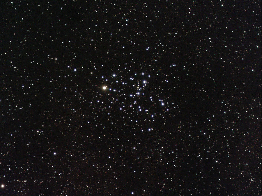
Welcome back to Messier Monday! We continue our tribute to our dear friend, Tammy Plotner, by looking at Messier 6, otherwise known as NGC 6405 and the Butterfly Cluster. Enjoy!
In the late 18th century, Charles Messier was busy hunting for comets in the night sky, and noticed several “nebulous” objects. After initially mistaking them for the comets he was seeking, he began to compile a list of these objects so other astronomers would not make the same mistake. Known as the Messier Catalog, this list consists of 100 objects, consisting of distant galaxies, nebulae, and star clusters.
This Catalog would go on to become a major milestone in the history of astronomy, as well as the study of Deep Sky Objects. Among the many famous objects in this catalog is M6 (aka. NGC 6405), an open cluster of stars in the constellation of Scorpius. Because of its vague resemblance to a butterfly, it is known as the Butterfly Cluster.