When it comes to scientists who revolutionized the way we think of the universe, few names stand out like Galileo Galilei. A noted inventor, physicist, engineer and astronomer, Galileo was one of the greatest contributors to the Scientific Revolution. He build telescopes, designed a compass for surveying and military use, created a revolutionary pumping system, and developed physical laws that were the precursors of Newton’s law of Universal Gravitation and Einstein’s Theory of Relativity.
But it was within the field of astronomy that Galileo made his most enduring impact. Using telescopes of his own design, he discovered Sunspots, the largest moons of Jupiter, surveyed The Moon, and demonstrated the validity of Copernicus’ heliocentric model of the universe. In so doing, he helped to revolutionize our understanding of the cosmos, our place in it, and helped to usher in an age where scientific reasoning trumped religious dogma.
Early Life:
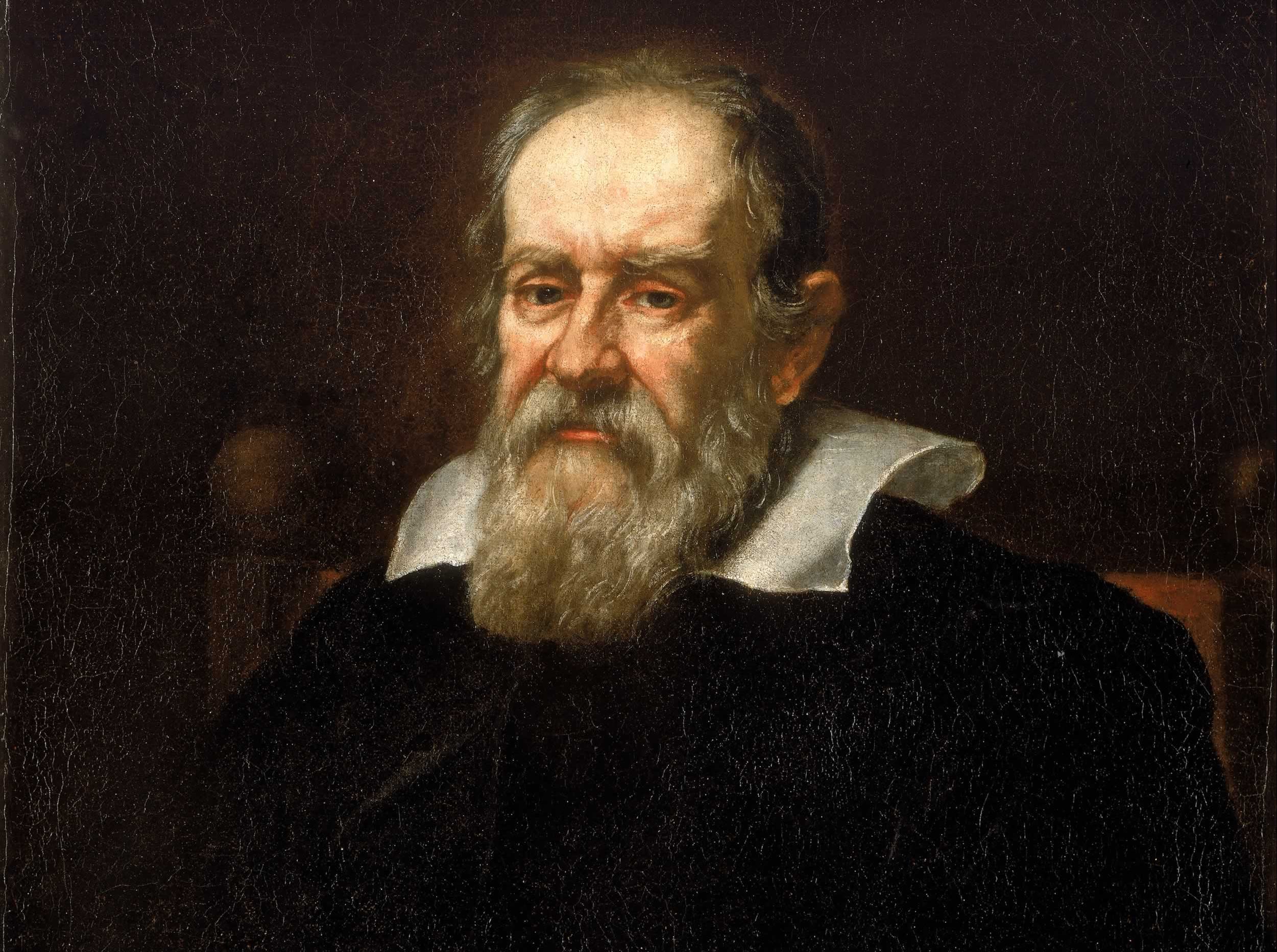
Galileo was born in Pisa, Italy, in 1564, into a noble but poor family. He was the first of six children of Vincenzo Galilei and Giulia Ammannati, who’s father also had three children out of wedlock. Galileo was named after an ancestor, Galileo Bonaiuti (1370 – 1450), a noted physician, university teacher and politician who lived in Florence.
His father, a famous lutenist, composer and music theorist, had a great impact on Galileo; transmitting not only his talent for music, but skepticism of authority, the value of experimentation, and the value of measures of time and rhythm to achieve success.
In 1572, when Galileo Galilei was eight, his family moved to Florence, leaving Galileo with his uncle Muzio Tedaldi (related to his mother through marriage) for two years.When he reached the age of ten, Galileo left Pisa to join his family in Florence and was tutored by Jacopo Borghini -a mathematician and professor from the university of Pisa.
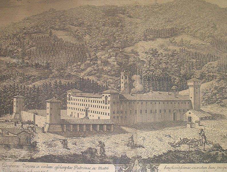
Once he was old enough to be educated in a monastery, his parents sent him to the Camaldolese Monastery at Vallombrosa, located 35 km southeast of Florence. The Order was independent from the Benedictines, and combined the solitary life of the hermit with the strict life of a monk. Galileo apparently found this life attractive and intending to join the Order, but his father insisted that he study at the University of Pisa to become a doctor.
Education:
While at Pisa, Galileo began studying medicine, but his interest in the sciences quickly became evident. In 1581, he noticed a swinging chandelier, and became fascinated by the timing of its movements. To him, it became clear that the amount of time, regardless of how far it was swinging, was comparable to the beating of his heart.
When he returned home, he set up two pendulums of equal length, swinging one with a large sweep and the other with a small sweep, and found that they kept time together. These observations became the basis of his later work with pendulums to keep time – work which would also be picked up almost a century later when Christiaan Huygens designed the first officially-recognized pendulum clock.
Shortly thereafter, Galileo accidentally attended a lecture on geometry, and talked his reluctant father into letting his study mathematics and natural philosophy instead of medicine. From that point onward, he began a steady processes of inventing, largely for the sake of appeasing his father’s desire for him to make money to pay off his siblings expenses (particularly those of his younger brother, Michelagnolo).
In 1589, Galileo was appointed to the chair of mathematics at the University of Pisa. In 1591, his father died, and he was entrusted with the care of his younger siblings. Being Professor of Mathematics at Pisa was not well paid, so Galileo lobbied for a more lucrative post. In 1592, this led to his appointment to the position of Professor of Mathematics at the University of Padua, where he taught Euclid’s geometry, mechanics, and astronomy until 1610.
During this period, Galileo made significant discoveries in both pure fundamental science as well as practical applied science. His multiple interests included the study of astrology, which at the time was a discipline tied to the studies of mathematics and astronomy. It was also while teaching the standard (geocentric) model of the universe that his interest in astronomy and the Copernican theory began to take off.
Telescopes:
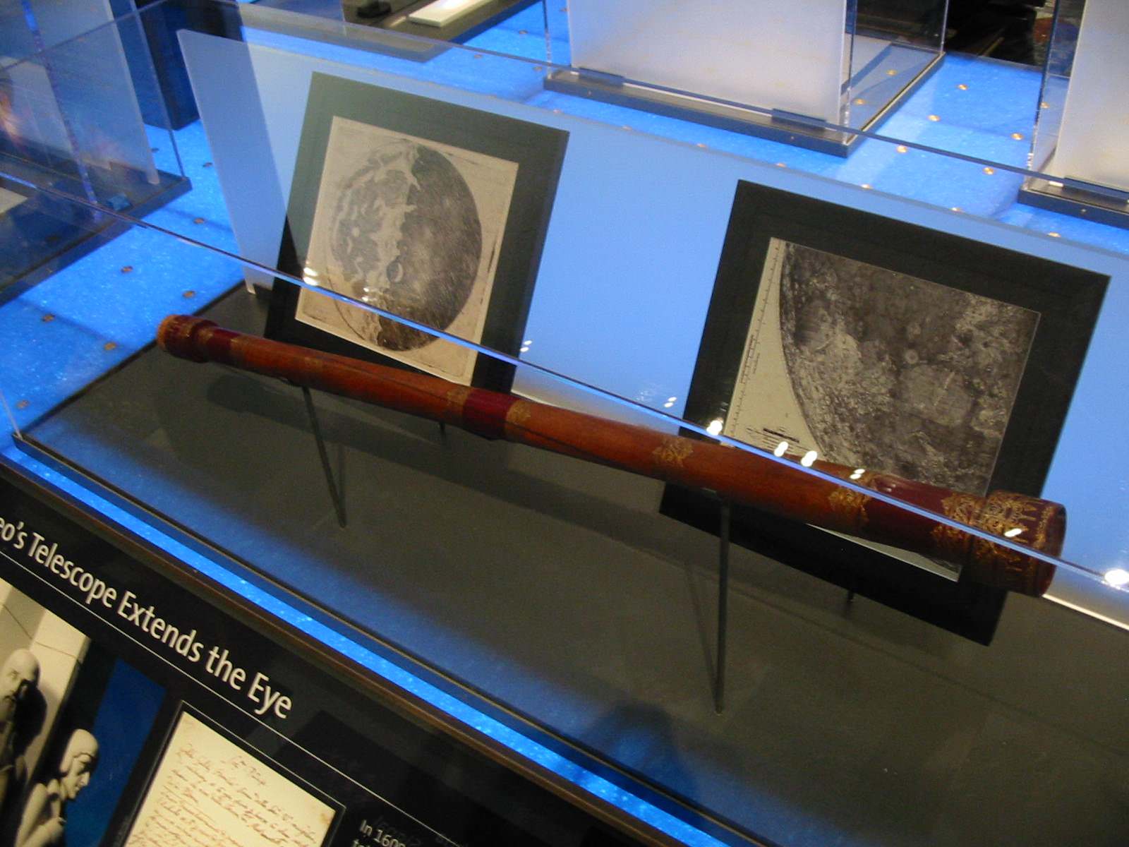
In 1609, Galileo received a letter telling him about a spyglass that a Dutchman had shown in Venice. Using his own technical skills as a mathematician and as a craftsman, Galileo began to make a series of telescopes whose optical performance was much better than that of the Dutch instrument.

As he would later write in his 1610 tract Sidereus Nuncius (“The Starry Messenger”):
“About ten months ago a report reached my ears that a certain Fleming had constructed a spyglass by means of which visible objects, though very distant from the eye of the observer, were distinctly seen as if nearby. Of this truly remarkable effect several experiences were related, to which some persons believed while other denied them. A few days later the report was confirmed by a letter I received from a Frenchman in Paris, Jacques Badovere, which caused me to apply myself wholeheartedly to investigate means by which I might arrive at the invention of a similar instrument. This I did soon afterwards, my basis being the doctrine of refraction.”
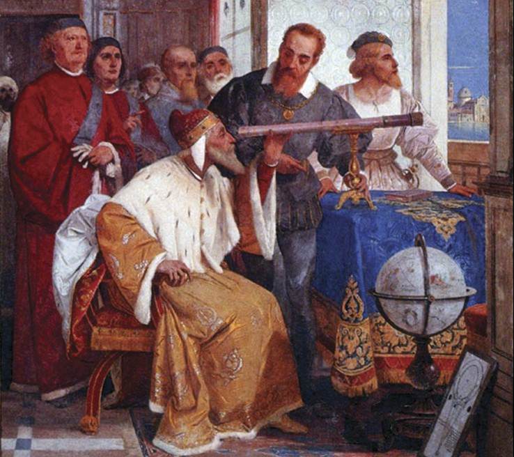
His first telescope – which he constructed between June and July of 1609 – was made from available lenses and had a three-powered spyglass. To improve upon this, Galileo learned how to grind and polish his own lenses. By August, he had created an eight-powered telescope, which he presented to the Venetian Senate.
By the following October or November, he managed to improve upon this with the creation a twenty-powered telescope. Galileo saw a great deal of commercial and military applications of his instrument(which he called a perspicillum) for ships at sea. However, in 1610, he began turning his telescope to the heavens and made his most profound discoveries.
Achievements in Astronomy:
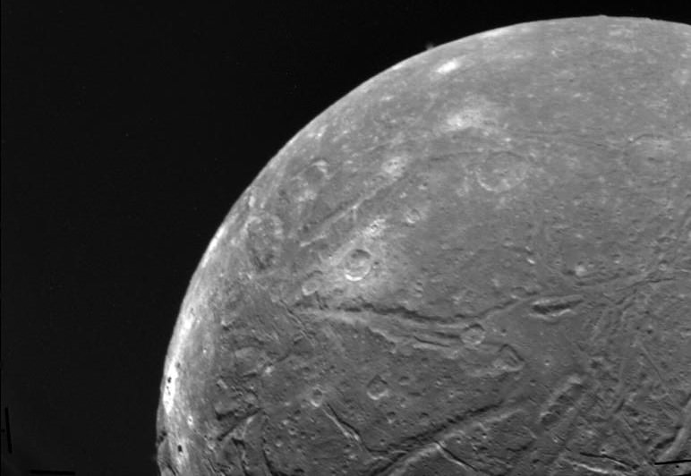
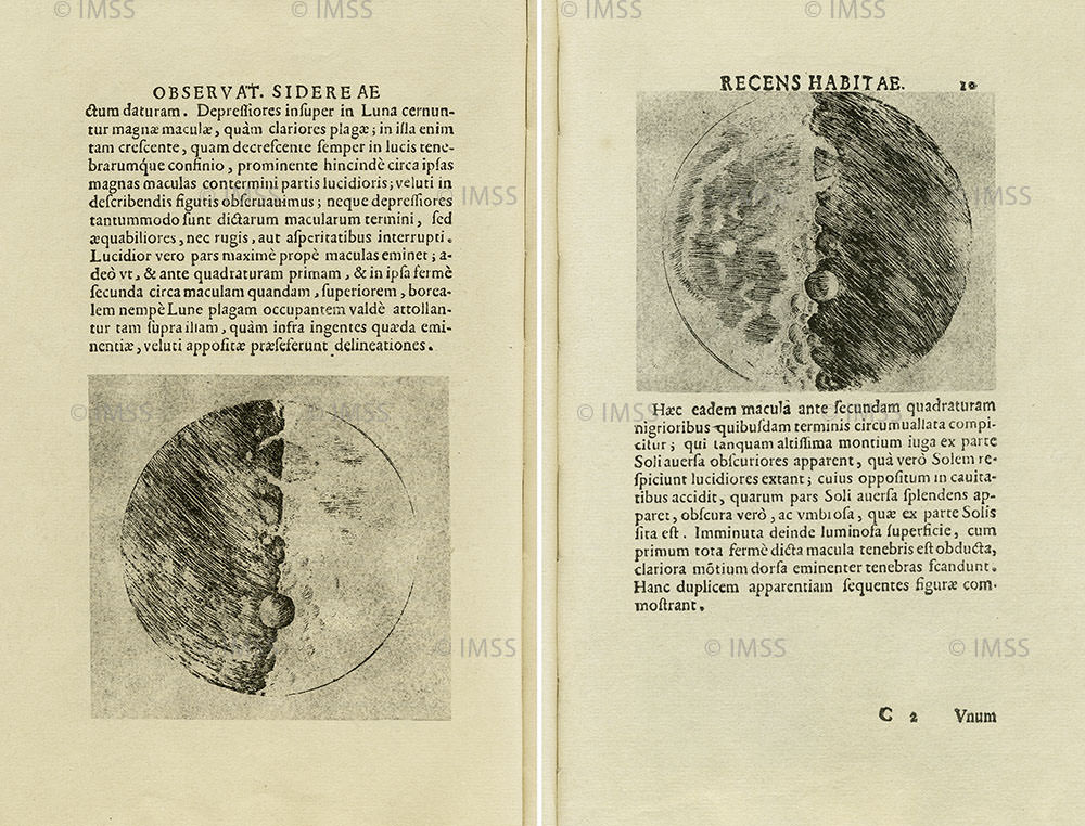
Using his telescope, Galileo began his career in astronomy by gazing at the Moon, where he discerned patterns of uneven and waning light. While not the first astronomer to do this, Galileo artistic’s training and knowledge of chiaroscuro – the use of strong contrasts between light and dark – allowed him to correctly deduce that these light patterns were the result of changes in elevation. Hence, Galileo was the first astronomer to discover lunar mountains and craters.
In The Starry Messenger, he also made topographical charts, estimating the heights of these mountains. In so doing, he challenged centuries of Aristotelian dogma that claimed that Moon, like the other planets, was a perfect, translucent sphere. By identifying that it had imperfections, in the forms of surface features, he began advancing the notion that the planets were similar to Earth.
Galileo also recorded his observations about the Milky Way in the Starry Messenger, which was previously believed to be nebulous. Instead, Galileo found that it was a multitude of stars packed so densely together that it appeared from a distance to look like clouds. He also reported that whereas the telescope resolved the planets into discs, the stars appeared as mere blazes of light, essentially unaltered in appearance by the telescope – thus suggesting that they were much farther away than previously thought.
Using his telescopes, Galileo also became one the first European astronomer to observe and study sunspots. Though there are records of previous instances of naked eye observations – such as in China (ca. 28 BCE), Anaxagoras in 467 BCE, and by Kepler in 1607 – they were not identifies as being imperfections on the surface of the Sun. In many cases, such as Kepler’s, it was thought that the spots were transits of Mercury.
In addition, there is also controversy over who was the first to observe sunspots during the 17th century using a telescope. Whereas Galileo is believed to have observed them in 1610, he did not publish about them and only began speaking to astronomers in Rome about them by the following year. In that time, German astronomer Christoph Scheiner had been reportedly observing them using a helioscope of his own design.
At around the same time, the Frisian astronomers Johannes and David Fabricius published a description of sunspots in June 1611. Johannes book, De Maculis in Sole Observatis (“On the Spots Observed in the Sun”) was published in autumn of 1611, thus securing credit for him and his father.
In any case, it was Galileo who properly identified sunspots as imperfections on the surface of the Sun, rather than being satellites of the Sun – an explanation that Scheiner, a Jesuit missionary, advanced in order to preserve his beliefs in the perfection of the Sun.
Using a technique of projecting the Sun’s image through the telescope onto a piece of paper, Galileo deduced that sunspots were, in fact, on the surface of the Sun or in its atmosphere. This presented another challenge to the Aristotelian and Ptolemaic view of the heavens, since it demonstrated that the Sun itself had imperfections.
On January 7th, 1610, Galileo pointed his telescope towards Jupiter and observed what he described in Nuncius as “three fixed stars, totally invisible by their smallness” that were all close to Jupiter and in line with its equator. Observations on subsequent nights showed that the positions of these “stars” had changed relative to Jupiter, and in a way that was not consistent with them being part of the background stars.

By January 10th, he noted that one had disappeared, which he attributed to it being hidden behind Jupiter. From this, he concluded that the stars were in fact orbiting Jupiter, and they were satellites of it. By January 13th, he discovered a fourth, and named them the Medicean stars, in honor of his future patron, Cosimo II de’ Medici, Grand Duke of Tuscany, and his three brothers.
Later astronomers, however, renamed them the Galilean Moons in honour of their discoverer. By the 20th century, these satellites would come to be known by their current names – Io, Europa, Ganymede, and Callisto – which had been suggested by 17th century German astronomer Simon Marius, apparently at the behest of Johannes Kepler.
Galileo’s observations of these satellites proved to be another major controversy. For the first time, a planet other than Earth was shown to have satellites orbiting it, which constituted yet another nail in the coffin of the geocentric model of the universe. His observations were independently confirmed afterwards, and Galileo continued to observe the satellites them and even obtained remarkably accurate estimates for their periods by 1611.
Heliocentrism:
Galileo’s greatest contribution to astronomy came in the form of his advancement of the Copernican model of the universe (i.e. heliocentrism). This began in 1610 with his publication of Sidereus Nuncius, which brought the issue of celestial imperfections before a wider audience. His work on sunspots and his observation of the Galilean Moons furthered this, revealing yet more inconsistencies in the currently accepted view of the heavens.
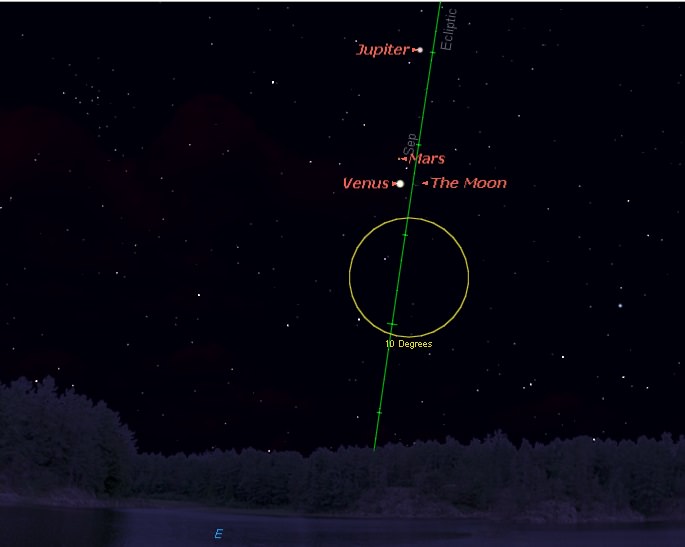
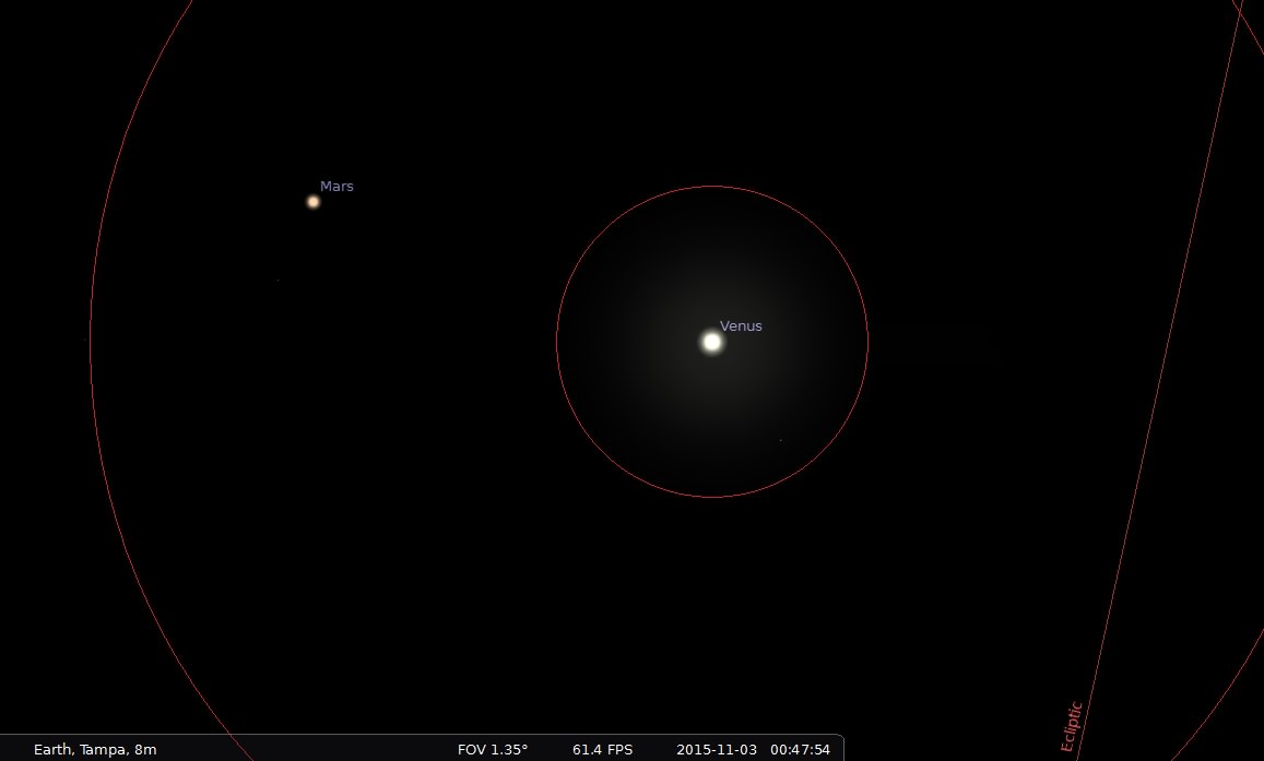
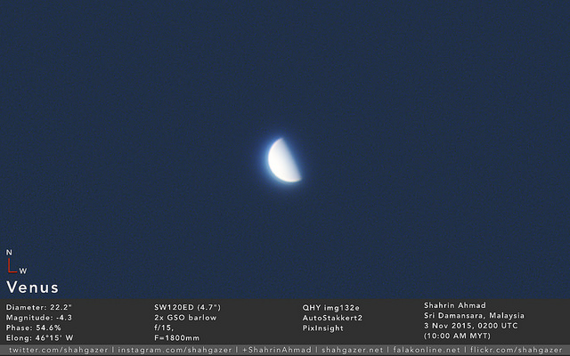
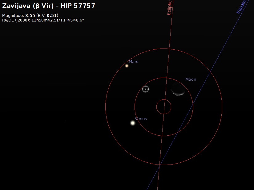
Other astronomical observations also led Galileo to champion the Copernican model over the traditional Aristotelian-Ptolemaic (aka. geocentric) view. From September 1610 onward, Galileo began observing Venus, noting that it exhibited a full set of phases similar to that of the Moon. The only explanation for this was that Venus was periodically between the Sun and Earth; while at other times, it was on the opposite side of the Sun.
According to the geocentric model of the universe, this should have been impossible, as Venus’ orbit placed it closer to Earth than the Sun – where it could only exhibit crescent and new phases. However, Galileo’s observations of it going through crescent, gibbous, full and new phases was consistent with the Copernican model, which established that Venus orbited the Sun within the Earth’s orbit.
These and other observations made the Ptolemaic model of the universe untenable. Thus, by the early 17th century, the great majority of astronomers began to convert to one of the various geo-heliocentric planetary models – such as the Tychonic, Capellan and Extended Capellan models. These all had the virtue of explaining problems in the geocentric model without engaging in the “heretical” notion that Earth revolved around the Sun.
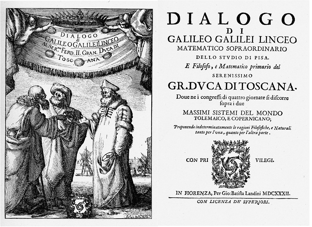
In 1632, Galileo addressed the “Great Debate” in his treatise Dialogo sopra i due massimi sistemi del mondo (Dialogue Concerning the Two Chief World Systems), in which he advocated the heliocentric model over the geocentric. Using his own telescopic observations, modern physics and rigorous logic, Galileo’s arguments effectively undermined the basis of Aristotle and Ptolemy’s system for a growing and receptive audience.
In the meantime, Johannes Kepler correctly identified the sources of tides on Earth – something which Galileo had become interesting in himself. But whereas Galileo attributed the ebb and flow of tides to the rotation of the Earth, Kepler ascribed this behavior to the influence of the Moon.
Combined with his accurate tables on the elliptical orbits of the planets (something Galileo rejected), the Copernican model was effectively proven. From the middle of the seventeenth century onward, there were few astronomers who were not Copernicans.
The Inquisition and House Arrest:
As a devout Catholic, Galileo often defended the heliocentric model of the universe using Scripture. In 1616, he wrote a letter to the Grand Duchess Christina, in which he argued for a non-literal interpretation of the Bible and espoused his belief in the heliocentric universe as a physical reality:
“I hold that the Sun is located at the center of the revolutions of the heavenly orbs and does not change place, and that the Earth rotates on itself and moves around it. Moreover … I confirm this view not only by refuting Ptolemy’s and Aristotle’s arguments, but also by producing many for the other side, especially some pertaining to physical effects whose causes perhaps cannot be determined in any other way, and other astronomical discoveries; these discoveries clearly confute the Ptolemaic system, and they agree admirably with this other position and confirm it.“
More importantly, he argued that the Bible is written in the language of the common person who is not an expert in astronomy. Scripture, he argued, teaches us how to go to heaven, not how the heavens go.

Initially, the Copernican model of the universe was not seen as an issue by the Roman Catholic Church or it’s most important interpreter of Scripture at the time – Cardinal Robert Bellarmine. However, in the wake of the Counter-Reformation, which began in 1545 in response to the Reformation, a more stringent attitude began to emerge towards anything seen as a challenge to papal authority.
Eventually, matters came to a head in 1615 when Pope Paul V (1552 – 1621) ordered that the Sacred Congregation of the Index (an Inquisition body charged with banning writings deemed “heretical”) make a ruling on Copernicanism. They condemned the teachings of Copernicus, and Galileo (who had not been personally involved in the trial) was forbidden to hold Copernican views.
However, things changed with the election of Cardinal Maffeo Barberini (Pope Urban VIII) in 1623. As a friend and admirer of Galileo’s, Barberini opposed the condemnation of Galileo, and gave formal authorization and papal permission for the publication of Dialogue Concerning the Two Chief World Systems.
However, Barberini stipulated that Galileo provide arguments for and against heliocentrism in the book, that he be careful not to advocate heliocentrism, and that his own views on the matter be included in Galileo’s book. Unfortunately, Galileo’s book proved to be a solid endorsement of heliocentrism and offended the Pope personally.
In it, the character of Simplicio, the defender of the Aristotelian geocentric view, is portrayed as an error-prone simpleton. To make matter worse, Galileo had the character Simplicio enunciate the views of Barberini at the close of the book, making it appear as though Pope Urban VIII himself was a simpleton and hence the subject of ridicule.
As a result, Galileo was brought before the Inquisition in February of 1633 and ordered to renounce his views. Whereas Galileo steadfastly defended his position and insisted on his innocence, he was eventually threatened with torture and declared guilty. The sentence of the Inquisition, delivered on June 22nd, contained three parts – that Galileo renounce Copernicanism, that he be placed under house arrest, and that the Dialogue be banned.
According to popular legend, after recanting his theory publicly that the Earth moved around the Sun, Galileo allegedly muttered the rebellious phrase: “E pur si muove” (“And yet it moves” in Latin). After a period of living with his friend, the Archbishop of Siena, Galileo returned to his villa at Arcetri (near Florence in 1634), where he spent the remainder of his life under house arrest.
Other Accomplishments:
In addition to his revolutionary work in astronomy and optics, Galileo is also credited with the invention of many scientific instruments and theories. Much of the devices he created were for the specific purpose of earning money to pay for his sibling’s expenses. However, they would also prove to have a profound impact in the fields of mechanics, engineering, navigation, surveying, and warfare.
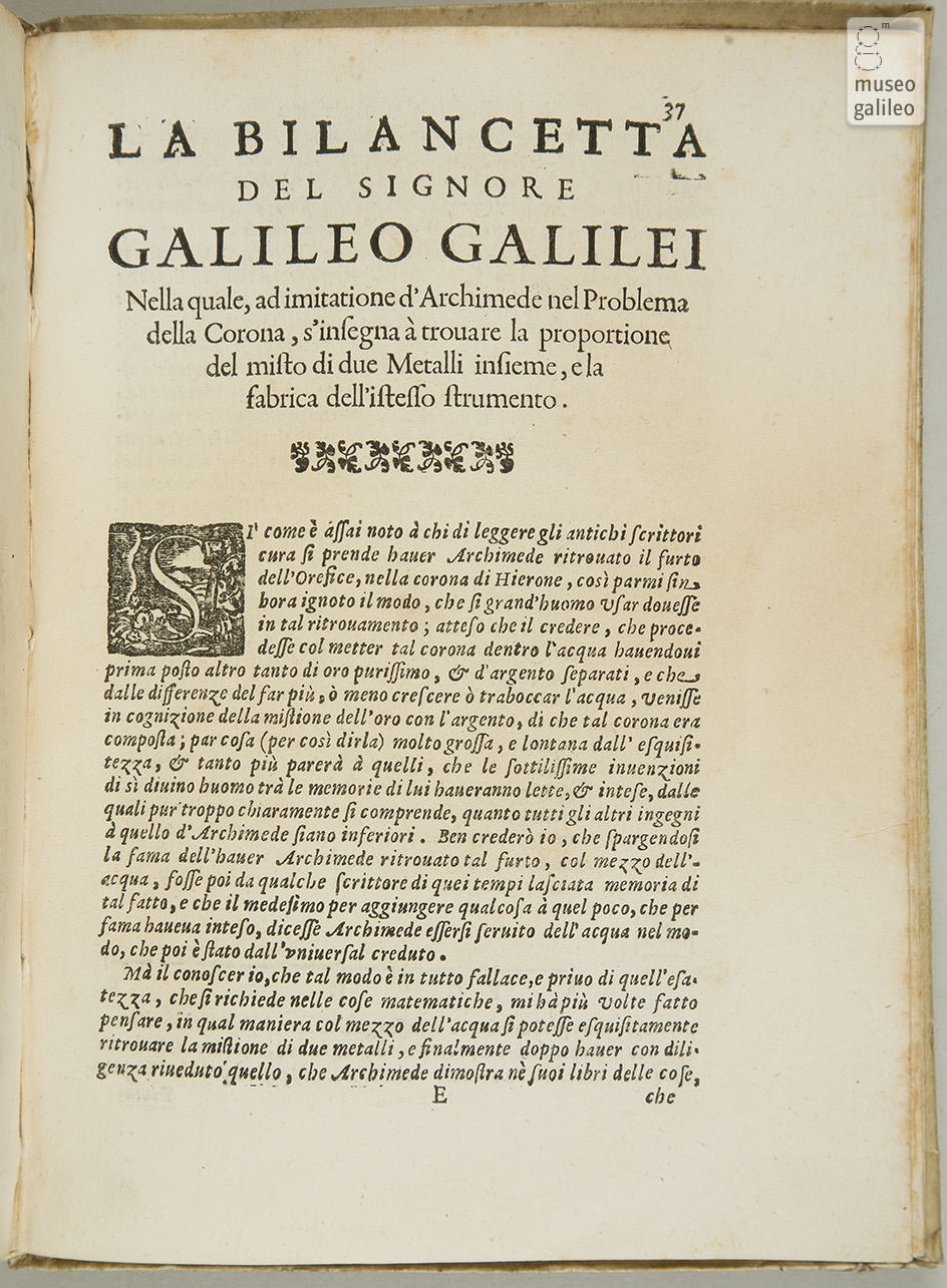
In 1586, at the age of 22, Galileo made his first groundbreaking invention. Inspired by the story of Archimedes and his “Eureka” moment, Galileo began looking into how jewelers weighed precious metals in air and then by displacement to determine their specific gravity. Working from this, he eventually theorized of a better method, which he described in a treatise entitled La Bilancetta (“The Little Balance”).
In this tract, he described an accurate balance for weighing things in air and water, in which the part of the arm on which the counter weight was hung was wrapped with metal wire. The amount by which the counterweight had to be moved when weighing in water could then be determined very accurately by counting the number of turns of the wire. In so doing, the proportion of metals like gold to silver in the object could be read off directly.
In 1592, when Galileo was a professor of mathematics at the University of Padua, he made frequent trips to the Arsenal – the inner harbor where Venetian ships were outfitted. The Arsenal had been a place of practical invention and innovation for centuries, and Galileo used the opportunity to study mechanical devices in detail.
In 1593, he was consulted on the placement of oars in galleys and submitted a report in which he treated the oar as a lever and correctly made the water the fulcrum. A year later the Venetian Senate awarded him a patent for a device for raising water that relied on a single horse for the operation. This became the basis of modern pumps.
To some, Galileo’s Pump was a merely an improvement on the Archimedes Screw, which was first developed in the third century BCE and patented in the Venetian Republic in 1567. However, there is no apparent evidence connecting Galileo’s invention to Archimedes’ earlier and less sophisticated design.
In ca. 1593, Galileo constructed his own version of a thermoscope, a forerunner of the thermometer, that relied on the expansion and contraction of air in a bulb to move water in an attached tube. Over time, he and his colleagues worked to develop a numerical scale that would measure the heat based on the expansion of the water inside the tube.
The cannon, which was first introduced to Europe in 1325, had become a mainstay of war by Galileo’s time. Having become more sophisticated and mobile, gunners needed instruments to help them coordinate and calculate their fire. As such, between 1595 and 1598, Galileo devised an improved geometric and military compass for use by gunners and surveyors.
During the 16th century, Aristotelian physics was still the predominant way of explaining the behavior of bodies near the Earth. For example, it was believed that heavy bodies sought their natural place of rest – i.e at the center of things. As a result, no means existed to explain the behavior of pendulums, where a heavy body suspended from a rope would swing back and forth and not seek rest in the middle.

Already, Galileo had conducted experiments that demonstrated that heavier bodies did not fall faster than lighter ones – another belief consistent with Aristotelian theory. In addition, he also demonstrated that objects thrown into the air travel in parabolic arcs. Based on this and his fascination with the back and forth motion of a suspended weight, he began to research pendulums in 1588.
In 1602, he explained his observations in a letter to a friend, in which he described the principle of isochronism. According to Galileo, this principle asserted that the time it takes for the pendulum to swing is not linked to the arc of the pendulum, but rather the pendulum’s length. Comparing two pendulum’s of similar length, Galileo demonstrated that they would swing at the same speed, despite being pulled at different lengths.
According to Vincenzo Vivian, one of Galileo’s contemporaries, it was in 1641 while under house arrest that Galileo created a design for a pendulum clock. Unfortunately, being blind at the time, he was unable to complete it before his death in 1642. As a result, Christiaan Huygens’ publication of Horologrium Oscillatorium in 1657 is recognized as the first recorded proposal for a pendulum clock.
Death and Legacy:
Galileo died on January 8th, 1642, at the age of 77, due to fever and heart palpitations that had taken a toll on his health. The Grand Duke of Tuscany, Ferdinando II, wished to bury him in the main body of the Basilica of Santa Croce, next to the tombs of his father and other ancestors, and to erect a marble mausoleum in his honor.
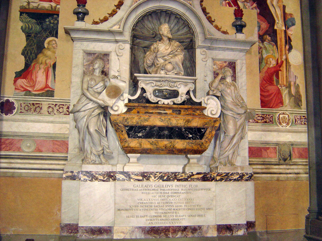
However, Pope Urban VIII objected on the basis that Galileo had been condemned by the Church, and his body was instead buried in a small room next to the novice’s chapel in the Basilica. However, after his death, the controversy surrounding his works and heliocentricm subsided, and the Inquisitions ban on his writing’s was lifted in 1718.
In 1737, his body was exhumed and reburied in the main body of the Basilica after a monument had been erected in his honor. During the exhumation, three fingers and a tooth were removed from his remains. One of these fingers, the middle finger from Galileo’s right hand, is currently on exhibition at the Museo Galileo in Florence, Italy.
In 1741, Pope Benedict XIV authorized the publication of an edition of Galileo’s complete scientific works which included a mildly censored version of the Dialogue. In 1758, the general prohibition against works advocating heliocentrism was removed from the Index of prohibited books, although the specific ban on uncensored versions of the Dialogue and Copernicus’s De Revolutionibus orbium coelestium (“On the Revolutions of the Heavenly Spheres“) remained.
All traces of official opposition to heliocentrism by the church disappeared in 1835 when works that espoused this view were finally dropped from the Index. And in 1939, Pope Pius XII described Galileo as being among the “most audacious heroes of research… not afraid of the stumbling blocks and the risks on the way, nor fearful of the funereal monuments”.

On October 31st, 1992, Pope John Paul II expressed regret for how the Galileo affair was handled, and issued a declaration acknowledging the errors committed by the Catholic Church tribunal. The affair had finally been put to rest and Galileo exonerated, though certain unclear statements issued by Pope Benedict XVI have led to renewed controversy and interest in recent years.
Alas, when it comes to the birth of modern science and those who helped create it, Galileo’s contributions are arguably unmatched. According to Stephen Hawking and Albert Einstein, Galileo was the father of modern science, his discoveries and investigations doing more to dispel the prevailing mood of superstition and dogma than anyone else in his time.
These include the discovery of craters and mountains on the Moon, the discovery of the four largest moons of Jupiter (Io, Europa, Ganymede and Callisto), the existence and nature of Sunspots, and the phases of Venus. These discoveries, combined with his logical and energetic defense of the Copernican model, made a lasting impact on astronomy and forever changed the way people look at the universe.
Galileo’s theoretical and experimental work on the motions of bodies, along with the largely independent work of Kepler and René Descartes, was a precursor of the classical mechanics developed by Sir Isaac Newton. His work with pendulums and time-keeping also previewed the work of Christiaan Huygens and the development of the pendulum clock, the most accurate timepiece of its day.
Galileo also put forward the basic principle of relativity, which states that the laws of physics are the same in any system that is moving at a constant speed in a straight line. This remains true, regardless of the system’s particular speed or direction, thus proving that there is no absolute motion or absolute rest. This principle provided the basic framework for Newton’s laws of motion and is central to Einstein’s special theory of relativity.
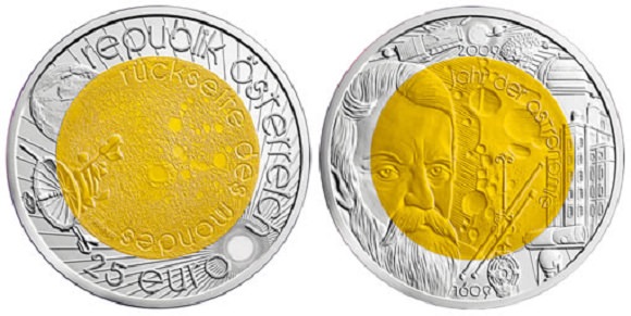
The United Nations chose 2009 to be the International Year of Astronomy, a global celebration of astronomy and its contributions to society and culture. The year 2009 was selected in part because it was the four-hundredth anniversary of Galileo first viewing the heavens with his a telescope he built himself.
A commemorative €25 coin was minted for the occasion, with the inset on the obverse side showing Galileo’s portrait and telescope, as well as one of his first drawings of the surface of the moon. In the silver circle that surrounds it, pictures of other telescopes – Isaac Newton’s Telescope, the observatory in Kremsmünster Abbey, a modern telescope, a radio telescope and a space telescope – are also shown.
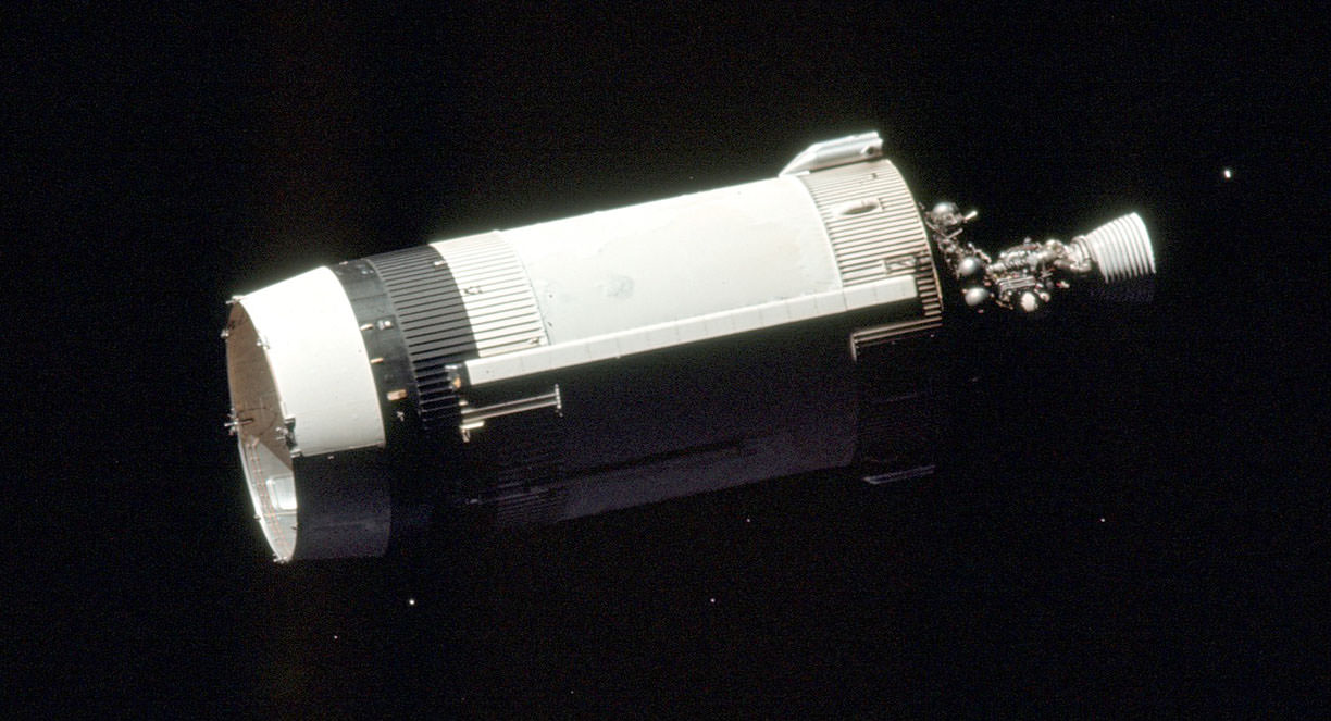
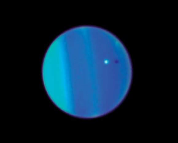
Other scientific endeavors and principles are named after Galileo, including the NASA Galileo spacecraft, which was the first spacecraft to enter orbit around Jupiter. Operating from 1989 to 2003, the mission consisted of an orbiter that observed the Jovian system, and an atmospheric probe that made the first measurements of Jupiter’s atmosphere.
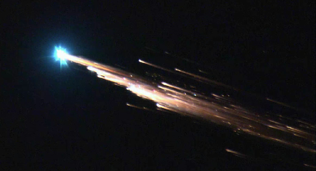
This mission found evidence of subsurface oceans on Europa, Ganymede and Callisto, and revealed the intensity of volcanic activity on Io. In 2003, the spacecraft was crashed into Jupiter’s atmosphere to avoid contamination of any of Jupiter’s moons.
The European Space Agency (ESA) is also developing a global satellite navigation system named Galileo. And in classical mechanics, the transformation between inertial systems is known as “Galilean Transformation“, which is denoted by the non-SI unit of acceleration Gal (sometimes known as the Galileo). Asteroid 697 Galilea is also named in his honor.
Yes, the sciences and humanity as a whole owes a great dept to Galileo. And as time goes on, and space exploration continues, it is likely we will continue to repay that debt by naming future missions – and perhaps even features on the Galilean Moons, should we ever settle there – after him. Seems like a small recompense for ushering in the age of modern science, no?
Universe Today has many interesting articles on Galileo, include the Galilean moons, Galileo’s inventions, and Galileo’s telescope.
For more information, check out the the Galileo Project and Galileo’s biography.
Astronomy Cast has an episode on choosing and using a telescope, and one which deals with the Galileo Spacecraft.