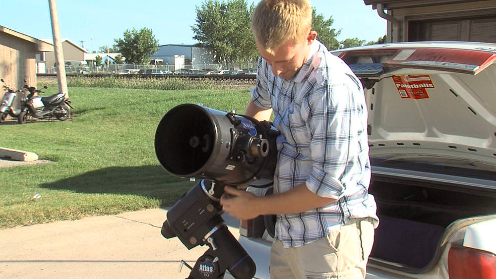
Levi Joraanstad, a student at North Dakota State University displays his telescope, which police mistook for a rifle. Image via WDAY TV, Fargo, North Dakota.
One more thing amateur astronomers might need to worry about besides clouds, bugs, and trying to fix equipment malfunctions in the dark – and this one’s a little more serious.
Earlier this week, two students at North Dakota State University (NDSU) in Fargo, North Dakota were settting up a telescope and camera system to take pictures of the Moon when armed police approached them. The police officers had mistaken the telescope for a rifle.
Students Levi Joraanstad and Colin Waldera told WDAY TV in Fargo that they were were setting up their telescope behind their apartment’s garage when they were blinded by a bright light and told to stop moving.
Initially, they thought it was a joke, that fellow students were pulling a prank, and because police were shining a bright light at them, the two students were blinded.
Police said that an officer patrolling the area had seen what he thought was suspicious activity behind the garage, thinking that one of the students’ dark sweater with white lettering on the back looked like a tactical vest, and that the telescope might be a rifle.
Police added that their response was a “better safe than sorry” approach, and they said the two students were never in any danger of being shot.
However, Joraanstad and Waldera said since they thought it was a joke, they initially ignored the order to stop moving and kept digging in their bags for equipment.
“I was kind of fumbling around with my stuff and my roommate and I were kind of talking, we were kind of wondering, what the heck’s going on? This is pretty dum that these guys are doing this,” WDAY quoted Joraanstad, a junior at NDSU. “And then they started shouting to quit moving or we could be shot. And so at that moment we kind of look at each other and we’re thinking we better take this seriously.”
If the police had acted more aggressively, the outcome could have been tragic. Joraanstad said the officers were very apologetic when they realized their mistake, and they explained what had happened.
So, watch where and how you point your telescope.
This is a rare occurrence, of course, and is nothing like risks amateur astronomers in Afghanistan regularly take to look through a telescope and share their views with local people. We wrote an article — which you can read here — about how they have to deal with more serious complications, such as making sure the area is clear of land mines, not arousing the suspicions the Taliban or the local police, and watching out for potential bombing raids by the US/UK/Afghan military alliance.
UPDATE: Maybe incidents like this aren’t quite as rare as I thought. Universe Today’s Bob King told me that just two weeks ago he was out observing in the countryside, when a very similar event happened to him. “A truck pulled up fast, with bright lights blinding my eyes and then the sheriff walked out of the car,” Bob said. “I quickly identified myself and explained what I was up to. He thought I was burying a dead body! No kidding.”
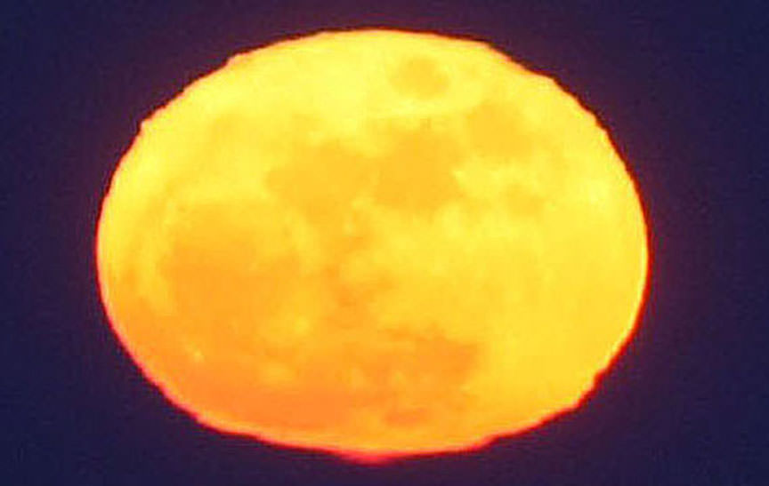
A Full Moon in all its horizontal glory. When near the horizon, refraction squeezes the lunar disk into an oval. Scattering removes the shorter wavelengths of white light, leaving the Moon a rich red or orange. Credit: Bob King
Who doesn’t love a Full Moon? Occurring about once a month, they never wear out their welcome. Each one becomes a special event to anticipate. In the summer months, when the Moon rises through the sultry haze, atmosphere and aerosols scatter away so much blue light and green light from its disk, the Moon glows an enticing orange or red.
At Full Moon, we’re also more likely to notice how the denser atmosphere near the horizon squeezes the lunar disk into a crazy hamburger bun shape. It’s caused by atmospheric refraction. Air closest to the horizon refracts more strongly than air near the top edge of the Moon, in effect “lifting” the bottom of the Moon up into the top. Squished light! We also get to see all the nearside maria or “seas” at full phase, while rayed craters like Tycho and Copernicus come into their full glory, looking for all the world like giant spatters of white paint even to the naked eye.
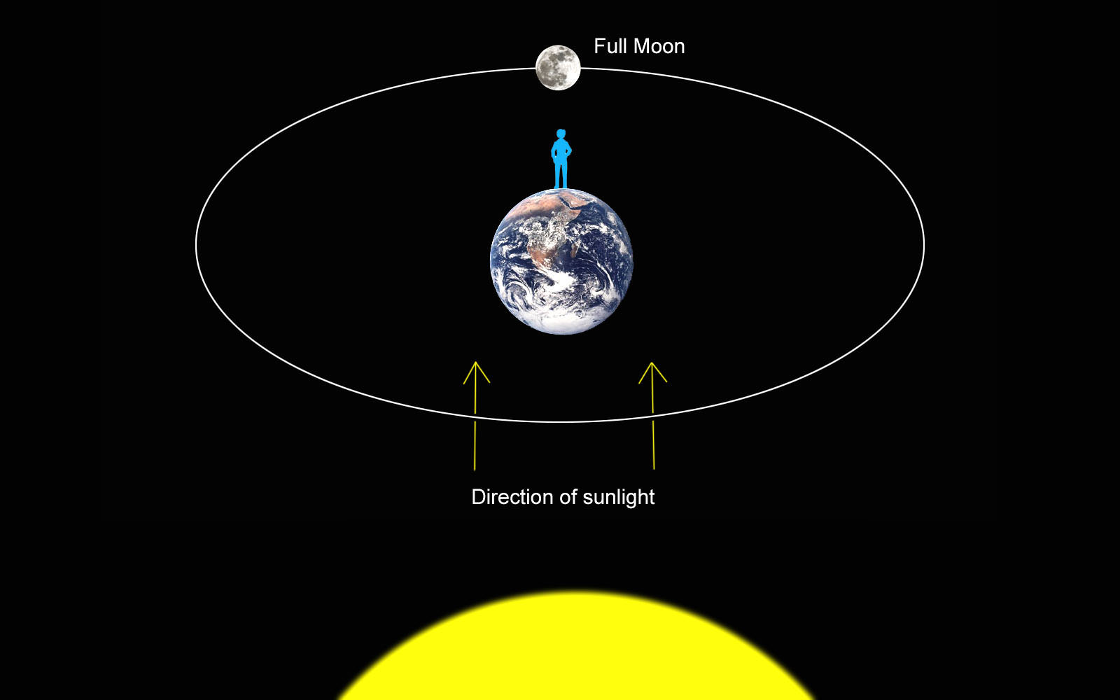
At full phase, the Moon lies directly opposite the Sun on the other side of Earth. Sunlight hits the Moon square on and fully illuminates the Earth-facing hemisphere. Credit: Bob King
Tomorrow night (August 29), the Full Sturgeon Moon rises around sunset across the world. The name comes from the association Great Lakes Indian groups made between the August moon and the best time to catch sturgeon. Next month’s moon is the familiar Harvest Moon; the additional light it provided at this important time of year allowed farmers to harvest into the night.
A Full Moon lies opposite the Sun in the sky exactly like a planet at opposition. Earth is stuck directly between the two orbs. As we look to the west to watch the Sun go down, the Moon creeps up at our back from the eastern horizon. Full Moon is the only time the Moon faces Sun directly – not off to one side or another – as seen from Earth, so the entire disk is illuminated.
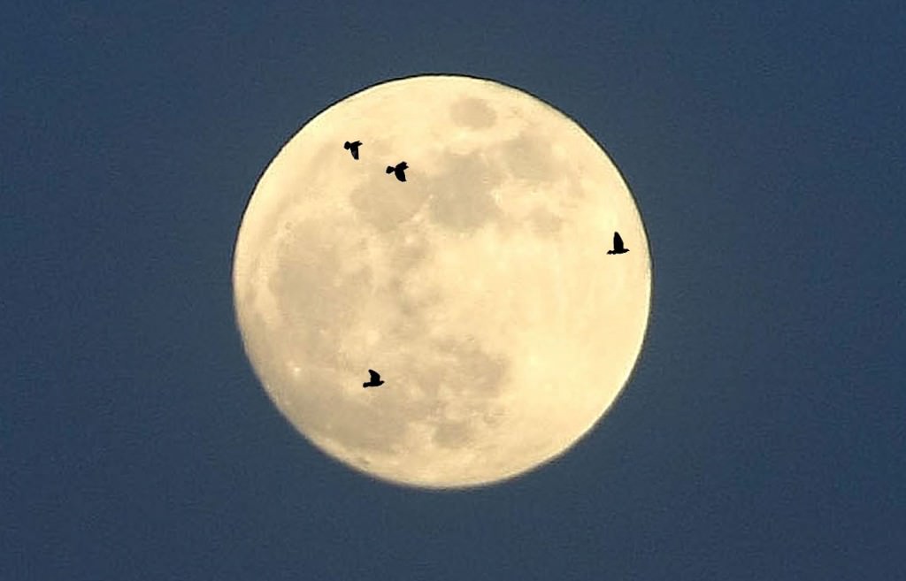
The moon provides the perfect backdrop for watching birds migrate at night. Although a small telescope is best, you might see an occasional bird in binoculars, too. Credit: Bob King
If you’re a moonrise watcher like I am, you’ll want to find a place where you can see all the way down to the eastern horizon tomorrow night. You’ll also need the time of moonrise for your city and a pair of binoculars. Sure, you can watch a moonrise without optical aid perfectly well, but you’ll miss all the cool distortions happening across the lunar disk from air turbulence. Birds have also begun their annual migration south. Don’t be surprised if your glass also shows an occasional winged silhouette zipping over those lunar seas.
Because the Moon’s orbit is tilted 5.1° with respect to Earth’s, it normally passes above or below Earth’s shadow with no eclipse — either lunar or solar. Only when the lineup is exact, does the Moon pass directly behind Earth and into its shadow. Credit: Bob King
Next month’s Full Moon is very special. A few times a year, the alignment of Sun, Earth and Moon (in that order) is precise, and the Full Moon dives into Earth’s shadow in total eclipse. That will happen overnight Sunday night-Monday morning September 27-28. This will be the final in the current tetradof four total lunar eclipses, each spaced about six months apart from the other. I think this one will be the best of the bunch. Why?
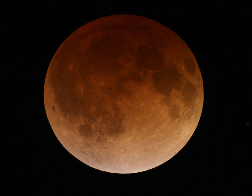
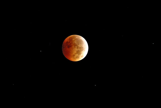
The totally eclipsed moon on April 15, 2014 from Duluth, Minn. This was the first in the series of four eclipses called a tetrad. September’s totally eclipsed Moon will appear similar. The coloring comes from sunlight grazing the edge of Earth’s atmosphere and refracted by it into the planet’s shadow. Credit: Bob King
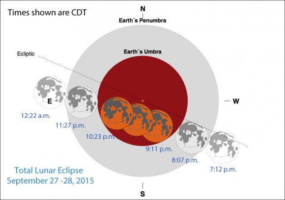
Convenient evening viewing hours (CDT times given) for observers in the Americas. Partial eclipse begins at 8:07 p.m., totality lasts from 9:11 – 10:23 p.m. and partial eclipse ends at 11:27 p.m. Those times mean that for many regions, kids can stay up and watch.
The Moon passes more centrally through Earth’s shadow than during the last total eclipse. That means a longer totality and possibly more striking color contrasts.
September’s will be the last total eclipse visible in the Americas until January 31, 2018. Between now and then, there will be a total of four minor penumbral eclipses and one small partial. Slim pickings.
Diagram showing the details of the upcoming total lunar eclipse. The event begins when the Moon treads into Earth’s outer shadow (penumbra) at 7:12 p.m. CDT. Partial phases start at 8:07 and totality at 9:11. Credit: NASA / Fred Espenak
Not only will the Americas enjoy a spectacle, but totality will also be visible from Europe, Africa and parts of Asia. For eastern hemisphere skywatchers, the event will occur during early morning hours of September 28. Universal or UT times for the eclipse are as follows: Partial phase begin at 1:07 a.m., totality from 2:11 – 3:23 a.m. with the end of partial phase at 4:27 a.m.
September 27-28, 2015 eclipse visibility map. Credit: NASA / Fred Espenak
We’ll have much more coverage on the upcoming eclipse in future articles here at Universe Today. I hope this brief look will serve to whet your appetite and help you anticipate what promises to be one of the best astronomical events of 2015.
The vast Kuiper Belt, which orbits at the outer edge of our Solar System, has been the site of many exciting discoveries in the past decade or so. Otherwise known as the Trans-Neptunian region, small bodies have been discovered here that have confounded our notions of what constitutes a planet and thrown our entire classification system for a loop. Of these, the most famous (and controversial) discovery was undoubtedly Eris.
First observed in 2005 by Mike Brown and his team, the discovery of Eris overturned decades of astronomical conventions. But both before and since then, many other “dwarf planets“, “plutoids” and “Trans-Neptunian Objects” (TNOs) have been found that further illustrated the need for reclassification. This includes the Kuiper Belt Object (KBO) 5000 Quaoar (or just Quaoar), which was actually discovered three years before Eris.
Discovery and Naming:
Quaoar was discovered on June 4th, 2002 by astronomers Chad Trujillo and Michael Brown of the California Institute of Technology, using images that were obtained with the Samuel Oschin Telescope at Palomar Observatory. The discovery was announced on October 7th, 2002, at a meeting of the American Astronomical Society. At the time, the object was designated as 2002 LM60, but would soon be renamed by Brown and Caltech his team.
Consistent with the IAU conventions for naming non-resonant Kuiper Belt Objects after creator deities, the object was given the name Quaoar after the Tongva creator god. The Tongva people (otherwise known as the Mission Indians) are native to the area around Los Angeles, where the discovery of Quaoar was made.
Images of Quaoar taken using the Oschin Telescope at the Palomar Observatory, California. Credit: Chad Trujillo & Michael Brown (Caltech)
Size, Mass and Orbit:
Given its distance, accurate measurements of Quaoar have been difficult to obtain. In 2004, Brown and Trujillo made direct measurements of the object with the Hubble Space Telescope and came up with an estimated diameter of 1260 ± 190 km.
However, these estimates were subsequently revised downward in 2013 by teams using a stellar occultation, and with data obtained with the Herschel Observatory’s PACS instrument and the Spectral and Photometric Imaging Receiver (SPIRE) at the University of Lethbridge, Alberta.
Combining this information, estimates of its diameter were then changed to between 1110 ± 5 km and 1074±38 km. By these estimates, Quaoar was the largest object to be discovered in the Solar System since the discovery of Pluto. However, it would later be supplanted by the discoveries of Eris, Haumea, and Makemake.
In addition, new techniques and a greater knowledge of KBOs led scientists to conclude that the 2004 HST size estimate for Quaoar was approximately 40% too large, and that a more proper estimate would be about 900 km. Using a weighted average of the SST and corrected HST estimates, Quaoar, as of 2010, is now believed to be about 890±70 km in diameter.
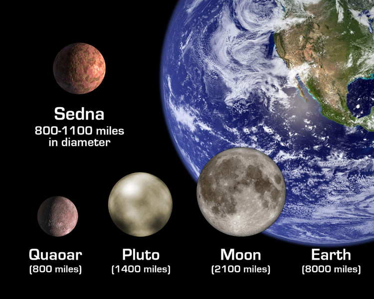
Given these dimensions, Quaoar is roughly one-twelfth the diameter of Earth, one third the diameter of the Moon, and half the size of Pluto. And with an estimated mass of 1.4 ± 0.1 × 10²¹ kg, Quaoar is about as massive as Pluto’s moon Charon, equivalent to 0.12 times the mass of Eris, and approximately 2.5 times as massive as Orcus.
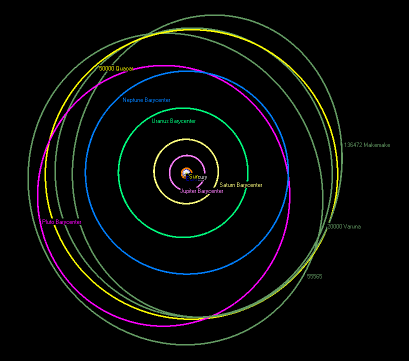
Quaoar orbit around the Sun varies slightly, ranging from 45.114 AU (6.75 x 10⁹ km / 4.19 x 10⁹ mi) at aphelion to 41.695 AU (6.24 x 10 km9/3.88 x 109 mi) at perihelion. Quaoar has an orbital period of 284.5 years, and a sidereal rotation period of about 17.68 hours.
Its orbit is also nearly circular and moderately inclined at approximately 8°, which is typical for the population of small classical KBOs, but exceptional among the large KBO. Pluto, Makemake, Haumea, Orcus, Varuna, and Salacia are all on highly inclined, more eccentric orbits.
At 43 AU and with a near-circular orbit, Quaoar is not significantly perturbed by Neptune; unlike Pluto, which is in 2:3 orbital resonance with Neptune. As of 2008, Quaoar was only 14 AU from Pluto, which made it the closest large body to the Pluto–Charon system. By Kuiper Belt standards this is very close.
The orbit of Quaoar (yellow) and various other cubewanos compared to the orbit of Neptune (blue) and Pluto (pink). Credit: Wikipedia Commons/kheider
Composition:
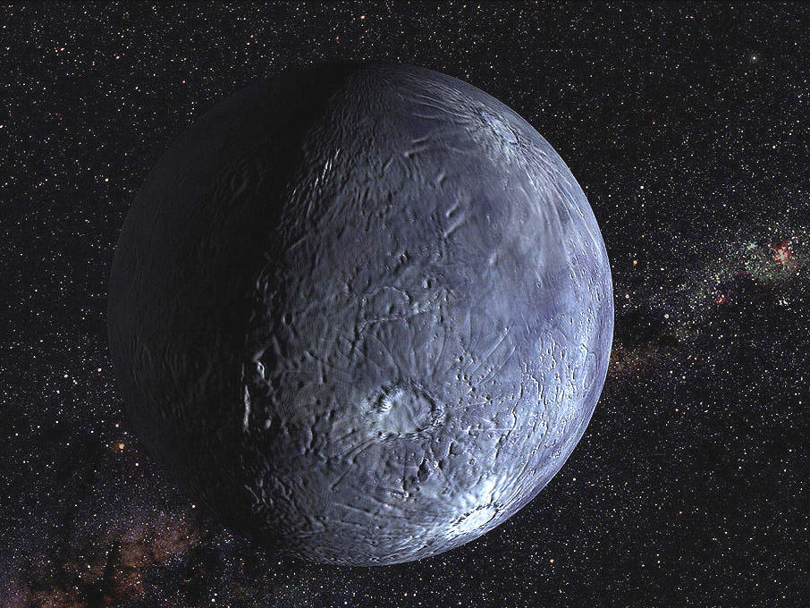
At the time of its discovery, not much was known about Kuiper belt objects. However, subsequent findings about this region have led scientists to conclude that the surface of Quaoar is likely to be highly similar to those of the icy satellites of Uranus and Neptune. This includes a low albedo, which could be as low as 0.1, which may be an indication that fresh ice has disappeared from its surface.
The surface is also moderately red, meaning that Quaoar is relatively more reflective in the red and near-infrared than in the blue. A 2006 model of internal heating via radioactive decay suggested that, unlike Orcus, Quaoar may not be capable of sustaining an internal ocean of liquid water at the mantle-core boundary.
Observations of Quaoar in the near infrared spectrum have indicated the presence of a small quantities of methane and ethane ice (about 5%). Scientists have also been surprised to find signs of crystalline ice on Quaoar, which is caused by sublimation and refreezing of water. This would indicate that the temperature rose to at least -160 °C (110 K or -260 °F) sometime in the last ten million years.
Artist’s impression of the size difference between Quaoar, Pluto, Sedna, Earth and the Moon. Credit: NASA/JPL-Caltech
Speculation as to what could have caused Quaoar to heat up from its natural temperature of -220 °C (55 K or -360 °F) have led to theories ranging from a barrage of mini-meteors that could have raised the temperature, to the presence of cryovolcanism. The latter theory, which is the more widely accepted one, holds that cryovolcanism occurred as a result of the decay of radioactive elements within Quaoar’s core.
Some scientist believe that Quaoar was nearly twice its current size before an ancient collision with another object, possibly Pluto, stripped it of its outer mantle. If true, it would mean that Quaoar once had more ice on its surface, and possibly a liquid water ocean at the core-mantle boundary.
Moon:
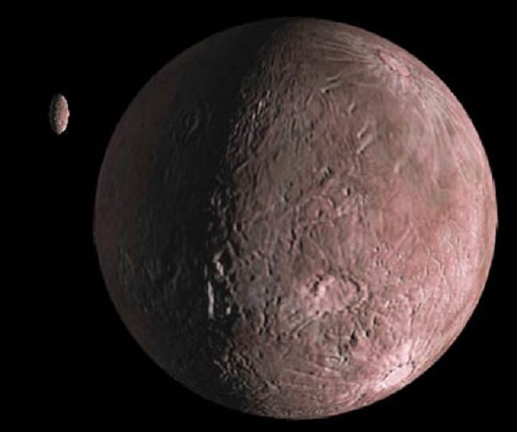
Quaoar has one known satellite, which was discovered on February 22nd, 2007. It orbits its primary at a distance of 14,500 km and has an orbital eccentricity of 0.14. Based on the assumption that the moon has the same albedo and density as Quaoar, the apparent magnitude of the moon indicates that it is 74 km in diameter and has 1/2000 the mass of Quaoar.
In terms of where it came from, Brown has suggested that it may be a remnant from a collision, which lost most of its mantle ice in the process. The choice for naming the moon was deferred to the Tongva people themselves, who selected the sky god Weymot, who is the son of Quaoar in Tongva mythology. The name became official on October 4th, 2009, with the publication of the Minor Planet Center’s latest issue.
Artist’s impression of the moderately red Quaoar and its moon Weywot. Credit: NASA/JPL-Caltech/R. Hurt (SSC-Caltech)
Classification:
According to the IAU, a dwarf planet is any celestial body that orbits a star, is massive enough to have become spherical under the power of its own gravity, but has not cleared its path of planetesimals, and is not the satellite of another object. Also, it must have enough mass to overcome its own compression and be in hydrostatic equilibrium.
Because Quaoar is a binary object, the mass of the system can be calculated from the orbit of the secondary. From this, Quaoar’s estimated density of 2.2 g/cm³ and its estimated diameter of 820 – 960 km suggest that it is large enough to be a dwarf planet.
This is based in part on estimates made by Mike Brown, who has claimed that rocky bodies around 900 km in diameter are sufficient to relax into hydrostatic equilibrium, whereas icy bodies can reach this state with diameters somewhere between 200 and 400 km.
In addition, Quaoar’s mass (which is believed to be greater than 1.6×10²¹ kg) is also greater than what the 2006 IAU draft definition of a planet claims is “usually” required for being in hydrostatic equilibrium (5×10²⁰ kg, 800 km). Light-curve-amplitude analysis shows only small deviations, suggesting that Quaoar is indeed a spheroid with small albedo spots.
Therefore, while it is not currently classified as a dwarf planet, it is considered a viable candidate. In the coming years, it may go on to join the ranks of Pluto, Eris, Haumea and Makemake as being officially recognized as such by the IAU and other astronomical bodies.
Exploration:
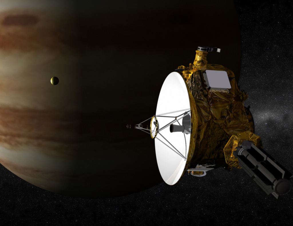
So far, no missions have been planned to Quaoar. While some have advocated sending the New Horizons mission to visit Quaoar and/or Sedna now that it’s flyby of Pluto is complete, NASA has declared this to be impossible. Much like Sedna, Quaoar is too far from the trajectory of the spacecraft, but also insists that both KBOs will be high on the list of candidate targets for future missions to the outer Solar System.
It has further been calculated that a flyby mission to Quaoar could take 13.57 years, using a Jupiter gravity assist and based on the launch dates of December 25th, 2016, November 22nd, 2027, December 22nd, 2028, January 22nd, 2030, or December 20thm, 2040. During any of these launch windows, Quaoar would be at a distance of 41 to 43 AU from the Sun by the time the spacecraft arrived.
In the meantime, all we can do is wait, and continue to observe Quaoar and its fellow Kuiper Belt Objects from afar. In the coming years, a decision is also likely to be made about whether or not it will be included on the list of the Solar System’s acknowledge dwarf planets.
We have written many articles about Quaoar for Universe Today. Here’s an article about the discovery of Quaoar, and here’s an article about the Kuiper Belt.
It seems as if the planets are fleeing the evening sky, just as the Fall school star party season is getting underway. Venus and Mars have entered the morning sky, and Jupiter reaches solar conjunction this week. Even glorious Saturn has passed eastern quadrature, and will soon depart evening skies.
Enter the ice giants, Uranus and Neptune. Both reach opposition for 2015 over the next two months, and the time to cross these two out solar system planets off your life list is now.
Looking east at dusk in late August, as Uranus and Neptune rise. Image credit: Stellarium
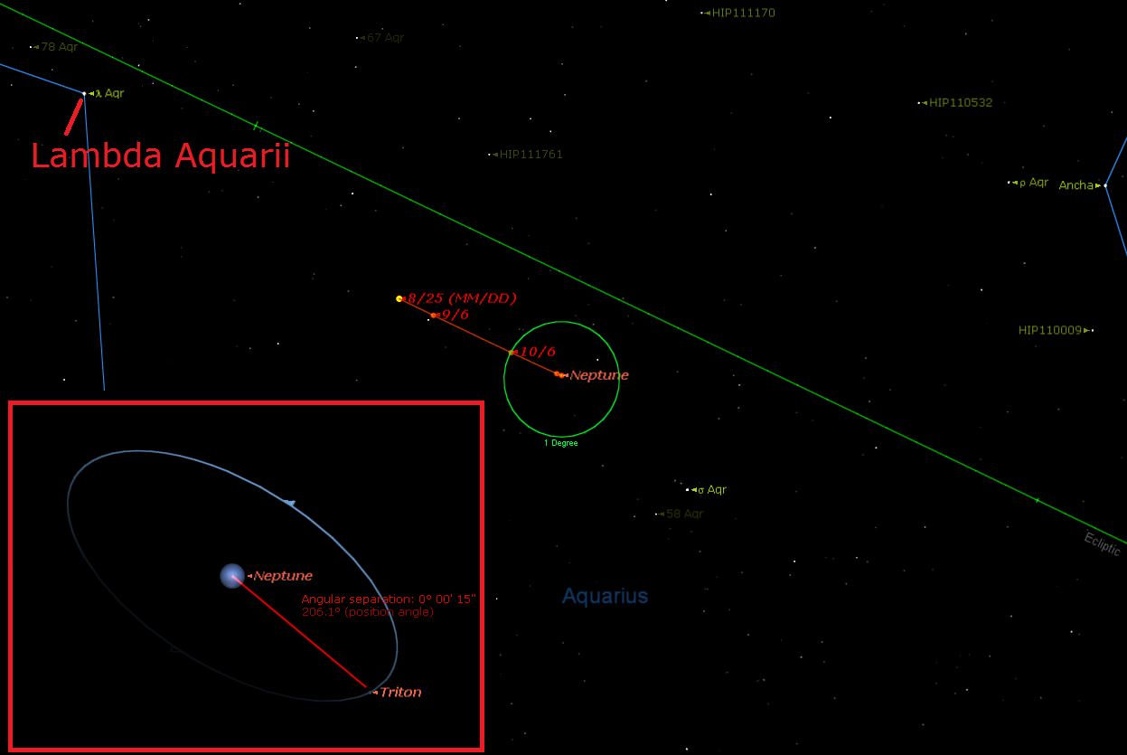
First up, the planet Neptune reaches opposition next week in the constellation Aquarius on the night of August 31st/September 1st. Shining at magnitude +7.8, Neptune spends the remainder of 2015 about three degrees southwest of the +3.7 magnitude star Lambda Aquarii. It’s possible to spot Neptune using binoculars, and about x100 magnification in a telescope eyepiece will just resolve the blue-grey 2.3 arc second disc of the planet. Though Neptune has 14 known moons, just one, Triton, is within reach of a backyard telescope. Triton shines at magnitude +13.5 (comparable to Pluto), and orbits Neptune in a retrograde path once every 6 days, getting a maximum of 15” from the disk of the planet.
The path of Neptune from late August through early November 2015. Inset: the position of Neptune’s moon Triton on the evening of August 31st: Image credit: Starry Night Education software
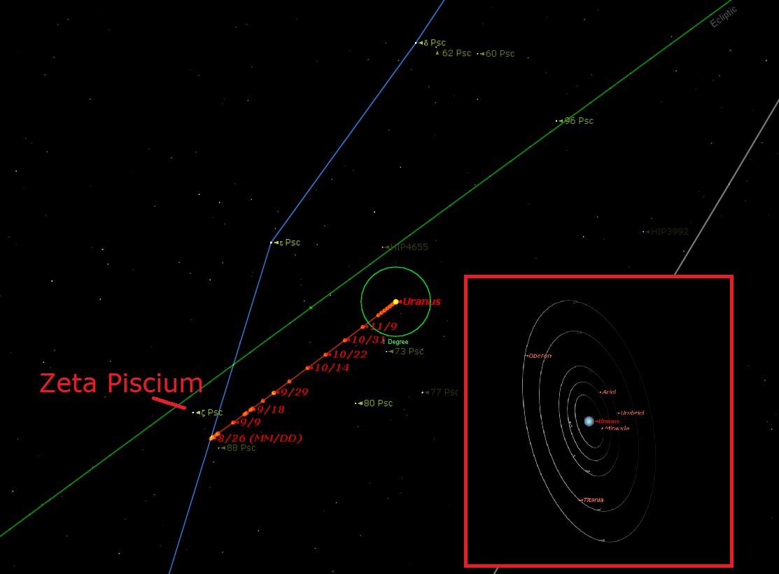
Uranus reaches opposition on October 11th in the adjacent constellation Pisces. Keep an eye on Uranus, as it nears the bright +5.2 magnitude star Zeta Piscium towards the end on 2015. Shining at magnitude +5.7 with a 3.6 arc second disk, Uranus hovers just on the edge of naked eye visibility from a dark sky site.
Uranus, left of the eclipsed Moon last October. Image credit and copyright: A Nartist
It’ll be worth hunting for Uranus on the night of September 27th/28th, when it sits 15 degrees east of the eclipsed Moon. Uranus turned up in many images of last Fall’s total lunar eclipse. This will be the final total lunar eclipse of the current tetrad, and the Moon will occult Uranus the evening after for the South Atlantic. This is part of a series of 19 ongoing occultations of Uranus by the Moon worldwide, which started in August 2014, and end on December 20th, 2015. After that, the Moon will move on and begin occulting Neptune next year in June through the end of 2017.
The visibility footprint of the September 29th occultation of Uranus by the Moon. Image credit: Occult 4.0.
Uranus has 27 known moons, four of which (Oberon, Ariel, Umbriel and Titania) are visible in a large backyard telescope. See our extensive article on hunting the moons of the solar system for more info, and the JPL/PDS rings node for corkscrew finder charts.
The path of Uranus, from late August through early December 2015. Inset: the position of the moons of Uranus on the evening of October 12th. Image credit: Starry Night Education software
The two outermost worlds have a fascinating entwined history. William Herschel discovered Uranus on the night of March 13th, 1781. We can be thankful that the proposed name ‘George’ after William’s benefactor King George the III didn’t stick. Herschel initially thought he’d discovered a comet, until he followed the slow motion of Uranus over several nights and realized that it had to be something large orbiting at a great distance from the Sun. Keep in mind, Uranus and Neptune both crept onto star charts unnoticed pre-1781. Galileo even famously sketched Neptune near Jupiter in 1612! Early astronomers simply considered the classical solar system out to Saturn as complete, end of story.
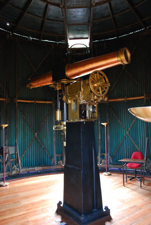
A classic 7″ Merz refractor at the Quito observatory, nearly identical to the instrument that first spied Neptune. Image Credit: Dave Dickinson
And the hunt was on. Astronomers soon realized that Uranus wasn’t staying put: something farther still from the Sun was tugging at its orbit. Mathematician Urbain Le Verrier predicted the position of the unseen planet, and on and on the night of September 23rd, 1846, astronomers at the Berlin observatory spied Neptune.
In a way, those early 19th century astronomers were lucky. Neptune and Uranus had just passed each other during a close encounter in 1821. Otherwise, Neptune might’ve remained hidden for several more decades. The synodic period of the two planets—that is, the time it takes the planets to return to opposition—differ by about 2-3 days. The very first documented conjunction of Neptune and Uranus occurred back in 1993, and won’t occur again until 2164. Heck, In 2010, Neptune completed its first orbit since discovery!
To date, only one mission, Voyager 2, has given us a close-up look at Uranus and Neptune during brief flybys. The final planetary encounter for Voyager 2 occurred in late August in 1989, when the spacecraft passed 4,800 kilometres (3,000 miles) above the north pole of Neptune.
All thoughts to ponder as you hunt for the outer ice giants. Sure, they’re tiny dots, but as with many nighttime treats, the ‘wow’ factor comes with just what you’re seeing, and the amazing story behind it.
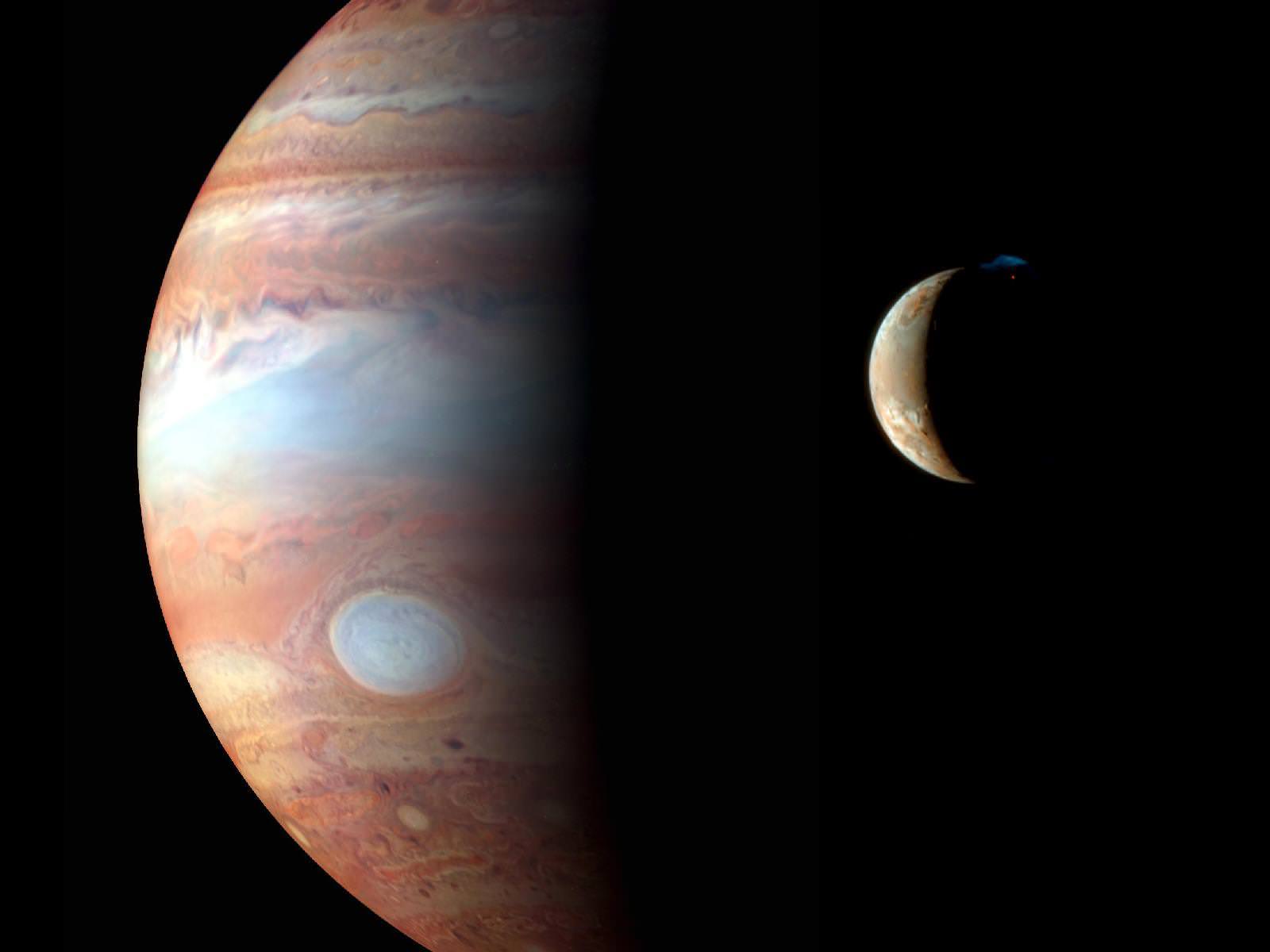
Ever since the invention of the telescope four hundred years ago, astronomers have been fascinated by the gas giant known as Jupiter. Between its constant, swirling clouds, its many, many moons, and its Giant Red Spot, there are many things about this planet that are both delightful and fascinating.
But perhaps the most impressive feature about Jupiter is its sheer size. In terms of mass, volume, and surface area, Jupiter is the biggest planet in our Solar System by a wide margin. And since people have been aware of its existence for thousands of years, it has played an active role in the cosmological systems many cultures. But just what makes Jupiter so massive, and what else do we know about it?
Size, Mass and Orbit:
Jupiter’s mass, volume, surface area and mean circumference are 1.8981 x 1027 kg, 1.43128 x 10¹⁵ km3, 6.1419 x 10¹⁰ km2, and 4.39264 x 10⁵ km respectively. To put that in perspective, Jupiter diameter is roughly 11 times that of Earth, and 2.5 the mass of all the other planets in the Solar System combined.
But, being a gas giant, it has a relatively low density – 1.326 g/cm3 – which is less than one quarter of Earth’s. This means that while Jupiter’s volume is equivalent to about 1,321 Earths, it is only 318 times as massive. The low density is one way scientists are able to determine that it is made mostly of gases, though the debate still rages on what exists at its core (see below).
Jupiter orbits the Sun at an average distance (semi-major axis) of 778,299,000 km (5.2 AU), ranging from 740,550,000 km (4.95 AU) at perihelion and 816,040,000 km (5.455 AU) at aphelion. At this distance, Jupiter takes 11.8618 Earth years to complete a single orbit of the Sun. In other words, a single Jovian year lasts the equivalent of 4,332.59 Earth days.
However, Jupiter’s rotation is the fastest of all the Solar System’s planets, completing a rotation on its axis in slightly less than ten hours (9 hours, 55 minutes and 30 seconds to be exact. Therefore, a single Jovian year lasts 10,475.8 Jovian solar days. This orbital period is two-fifths that of Saturn, which means that the two largest planets in our Solar System form a 5:2 orbital resonance.
Structure and Composition:
Jupiter is composed primarily of gaseous and liquid matter. It is the largest of the gas giants, and like them, is divided between a gaseous outer atmosphere and an interior that is made up of denser materials. It’s upper atmosphere is composed of about 88–92% hydrogen and 8–12% helium by percent volume of gas molecules, and approx. 75% hydrogen and 24% helium by mass, with the remaining one percent consisting of other elements.
This cut-away illustrates a model of the interior of Jupiter, with a rocky core overlaid by a deep layer of liquid metallic hydrogen. Credit: Kelvinsong/Wikimedia Commons
The atmosphere contains trace amounts of methane, water vapor, ammonia, and silicon-based compounds as well as trace amounts of benzene and other hydrocarbons. There are also traces of carbon, ethane, hydrogen sulfide, neon, oxygen, phosphine, and sulfur. Crystals of frozen ammonia have also been observed in the outermost layer of the atmosphere.
The interior contains denser materials, such that the distribution is roughly 71% hydrogen, 24% helium and 5% other elements by mass. It is believed that Jupiter’s core is a dense mix of elements – a surrounding layer of liquid metallic hydrogen with some helium, and an outer layer predominantly of molecular hydrogen. The core has also been described as rocky, but this remains unknown as well.
In 1997, the existence of the core was suggested by gravitational measurements, indicating a mass of from 12 to 45 times the Earth’s mass, or roughly 4%–14% of the total mass of Jupiter. The presence of a core is also supported by models of planetary formation that indicate how a rocky or icy core would have been necessary at some point in the planet’s history in order to collect all of its hydrogen and helium from the protosolar nebula.
However, it is possible that this core has since shrunk due to convection currents of hot, liquid, metallic hydrogen mixing with the molten core. This core may even be absent now, but a detailed analysis is needed before this can be confirmed. The Juno mission, which launched in August 2011 (see below), is expected to provide some insight into these questions, and thereby make progress on the problem of the core.
The temperature and pressure inside Jupiter increase steadily toward the core. At the “surface”, the pressure and temperature are believed to be 10 bars and 340 K (67 °C, 152 °F). At the “phase transition” region, where hydrogen becomes metallic, it is believed the temperature is 10,000 K (9,700 °C; 17,500 °F) and the pressure is 200 GPa. The temperature at the core boundary is estimated to be 36,000 K (35,700 °C; 64,300 °F) and the interior pressure at roughly 3,000–4,500 GPa.
Jupiter’s Moons:
The Jovian system currently includes 67 known moons. The four largest are known as the Galilean Moons, which are named after their discoverer, Galileo Galilei. They include: Io, the most volcanically active body in our Solar System; Europa, which is suspected of having a massive subsurface ocean; Ganymede, the largest moon in our Solar System; and Callisto, which is also thought to have a subsurface ocean and features some of the oldest surface material in the Solar System.
Then there’s the Inner Group (or Amalthea group), which is made up of four small moons that have diameters of less than 200 km, orbit at radii less than 200,000 km, and have orbital inclinations of less than half a degree. This groups includes the moons of Metis, Adrastea, Amalthea, and Thebe. Along with a number of as-yet-unseen inner moonlets, these moons replenish and maintain Jupiter’s faint ring system.
Jupiter also has an array of Irregular Satellites, which are substantially smaller and have more distant and eccentric orbits than the others. These moons are broken down into families that have similarities in orbit and composition, and are believed to be largely the result of collisions from large objects that were captured by Jupiter’s gravity.
Illustration of Jupiter and the Galilean satellites. Credit: NASA
Atmosphere and Storms:
Much like Earth, Jupiter experiences auroras near its northern and southern poles. But on Jupiter, the auroral activity is much more intense and rarely ever stops. The intense radiation, Jupiter’s magnetic field, and the abundance of material from Io’s volcanoes that react with Jupiter’s ionosphere create a light show that is truly spectacular.
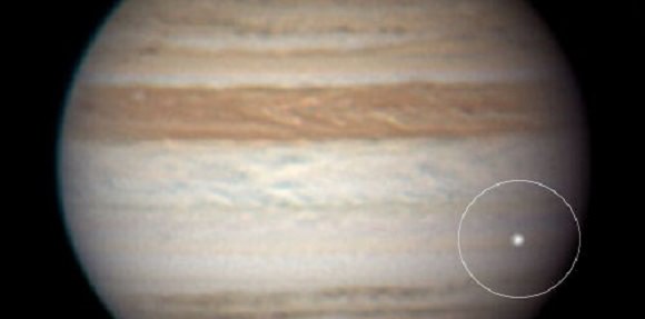
Jupiter also experiences violent weather patterns. Wind speeds of 100 m/s (360 km/h) are common in zonal jets, and can reach as high as 620 kph (385 mph). Storms form within hours and can become thousands of km in diameter overnight. One storm, the Great Red Spot, has been raging since at least the late 1600s. The storm has been shrinking and expanding throughout its history; but in 2012, it was suggested that the Giant Red Spot might eventually disappear.
Jupiter is perpetually covered with clouds composed of ammonia crystals and possibly ammonium hydrosulfide. These clouds are located in the tropopause and are arranged into bands of different latitudes, known as “tropical regions”. The cloud layer is only about 50 km (31 mi) deep, and consists of at least two decks of clouds: a thick lower deck and a thin clearer region.
There may also be a thin layer of water clouds underlying the ammonia layer, as evidenced by flashes of lightning detected in the atmosphere of Jupiter, which would be caused by the water’s polarity creating the charge separation needed for lightning. Observations of these electrical discharges indicate that they can be up to a thousand times as powerful as those observed here on the Earth.
A color composite image of the June 3rd Jupiter impact flash. Credit: Anthony Wesley
Historical Observations of the Planet:
As a planet that can be observed with the naked eye, humans have known about the existence of Jupiter for thousands of years. It has therefore played a vital role in the mythological and astrological systems of many cultures. The first recorded mentions of it date back to the Babylon Empire of the 7th and 8th centuries BCE.
In the 2nd century, the Greco-Egyptian astronomer Ptolemy constructed his famous geocentric planetary model that contained deferents and epicycles to explain the orbit of Jupiter relative to the Earth (i.e. retrograde motion). In his work, the Almagest, he ascribed an orbital period of 4332.38 days to Jupiter (11.86 years).
In 499, Aryabhata – a mathematician-astronomer from the classical age of India – also used a geocentric model to estimate Jupiter’s period as 4332.2722 days, or 11.86 years. It has also been ventured that the Chinese astronomer Gan De discovered Jupiter’s moons in 362 BCE without the use of instruments. If true, it would mean that Galileo was not the first to discovery the Jovian moons two millennia later.
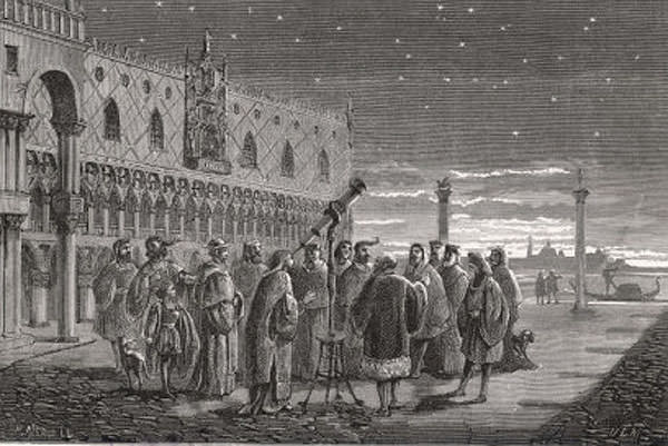
In 1610, Galileo Galilei was the first astronomer to use a telescope to observe the planets. In the course of his examinations of the outer Solar System, he discovered the four largest moons of Jupiter (now known as the Galilean Moons). The discovery of moons other than Earth’s was a major point in favor of Copernicus’heliocentric theory of the motions of the planets.
Galileo shows of the sky in Saint Mark’s square in Venice. Note the lack of adaptive optics. Credit: Public Domain
During the 1660s, Cassini used a new telescope to discover Jupiter’s spots and colorful bands and observed that the planet appeared to be an oblate spheroid. By 1690, he was also able to estimate the rotation period of the planet and noticed that the atmosphere undergoes differential rotation. In 1831, German astronomer Heinrich Schwabe produced the earliest known drawing to show details of the Great Red Spot.
In 1892, E. E. Barnard observed a fifth satellite of Jupiter using the refractor telescope at the Lick Observatory in California. This relatively small object was later named Amalthea, and would be the last planetary moon to be discovered directly by visual observation.
In 1932, Rupert Wildt identified absorption bands of ammonia and methane in the spectra of Jupiter; and by 1938, three long-lived anticyclonic features termed “white ovals” were observed. For several decades, they remained as separate features in the atmosphere, sometimes approaching each other but never merging. Finally, two of the ovals merged in 1998, then absorbed the third in 2000, becoming Oval BA.
Beginning in the 1950s, radiotelescopic research of Jupiter began. This was due to astronomers Bernard Burke and Kenneth Franklin’s detection of radio signals coming from Jupiter in 1955. These bursts of radio waves, which corresponded to the rotation of the planet, allowed Burke and Franklin to refine estimates of the planet’s rotation rate.
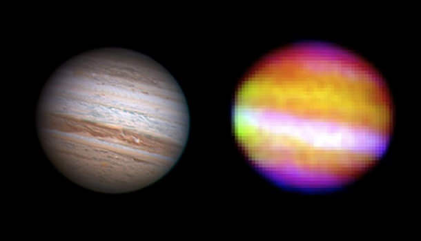
Infrared image of Jupiter from SOFIA’s First Light flight composed of individual images at wavelengths made by Cornell University’s FORCAST camera. Credit: Anthony Wesley/Cornell University
Over time, scientists discovered that there were three forms of radio signals transmitted from Jupiter – decametric radio bursts, decimetric radio emissions, and thermal radiation. Decametric bursts vary with the rotation of Jupiter, and are influenced by the interaction of Io with Jupiter’s magnetic field.
Decimetric radio emissions – which originate from a torus-shaped belt around Jupiter’s equator – are caused by cyclotronic radiation from electrons that are accelerated in Jupiter’s magnetic field. Meanwhile, thermal radiation is produced by heat in the atmosphere of Jupiter. Visualizations of Jupiter using radiotelescopes have allowed astronomers to learn much about its atmosphere, thermal properties and behavior.
Exploration:
Since 1973, a number of automated spacecraft have been sent to the Jovian system and performed planetary flybys that brought them within range of the planet. The most notable of these was Pioneer 10, the first spacecraft to get close enough to send back photographs of Jupiter and its moons. Between this mission and Pioneer 11, astronomers learned a great deal about the properties and phenomena of this gas giant.
Artist impression of Pioneer 10 at Jupiter. Image credit: NASA/JPL
For example, they discovered that the radiation fields near the planet were much stronger than expected. The trajectories of these spacecraft were also used to refine the mass estimates of the Jovian system, and radio occultations by the planet resulted in better measurements of Jupiter’s diameter and the amount of polar flattening.
Six years later, the Voyager missions began, which vastly improved the understanding of the Galilean moons and discovered Jupiter’s rings. They also confirmed that the Great Red Spot was anticyclonic, that its hue had changed sine the Pioneer missions – turning from orange to dark brown – and spotted lightning on its dark side. Observations were also made of Io, which showed a torus of ionized atoms along its orbital path and volcanoes on its surface.
On December 7th, 1995, the Galileo orbiter became the first probe to establish orbit around Jupiter, where it would remain for seven years. During its mission, it conducted multiple flybys of all the Galilean moons and Amalthea and deployed an probe into the atmosphere. It was also in the perfect position to witness the impact of Comet Shoemaker–Levy 9 as it approached Jupiter in 1994.
On September 21st, 2003, Galileo was deliberately steered into the planet and crashed in its atmosphere at a speed of 50 km/s, mainly to avoid crashing and causing any possible contamination to Europa – a moon which is believed to harbor life.
Artist impression of New Horizons with Jupiter. Image credit: NASA/JPL/JHUAPL
Data gathered by both the probe and orbiter revealed that hydrogen composes up to 90% of Jupiter’s atmosphere. The temperatures data recorded was more than 300 °C (570 °F) and the wind speed measured more than 644 kmph (400 mph) before the probe vaporized.
In 2000, the Cassini probe (while en route to Saturn) flew by Jupiter and provided some of the highest-resolution images ever taken of the planet. While en route to Pluto, the New Horizons space probe flew by Jupiter and measured the plasma output from Io’s volcanoes, studied all four Galileo moons in detail, and also conducting long-distance observations of Himalia and Elara.
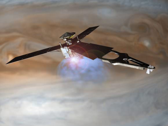
NASA’s Juno mission, which launched in August 2011, achieved orbit around the Jovian planet on July 4th, 2016. The purpose of this mission to study Jupiter’s interior, its atmosphere, its magnetosphere and gravitational field, ultimately for the purpose of determining the history of the planet’s formation (which will shed light on the formation of the Solar System).
As the probe entered its polar elliptical orbit on July 4th after completing a 35-minute-long firing of the main engine, known as Jupiter Orbital Insertion (or JOI). As the probe approached Jupiter from above its north pole, it was afforded a view of the Jovian system, which it took a final picture of before commencing JOI.
Illustration of NASA’s Juno spacecraft firing its main engine to slow down and go into orbit around Jupiter. Credit: NASA/Lockheed Martin
On July 10th, the Juno probe transmitted its first imagery from orbit after powering back up its suite of scientific instruments. The images were taken when the spacecraft was 4.3 million km (2.7 million mi) from Jupiter and on the outbound leg of its initial 53.5-day capture orbit. The color image shows atmospheric features on Jupiter, including the famous Great Red Spot, and three of the massive planet’s four largest moons – Io, Europa and Ganymede, from left to right in the image.
The next planned mission to the Jovian system will be performed by the European Space Agency’s Jupiter Icy Moon Explorer (JUICE), due to launch in 2022, followed by NASA’s Europa Clipper mission in 2025.
Exoplanets:
The discovery of exoplanets has revealed that planets can get even bigger than Jupiter. In fact, the number of “Super Jupiters” observed by the Kepler space probe (as well as ground-based telescopes) in the past few years has been staggering. In fact, as of 2015, more than 300 such planets have been identified.
Notable examples include PSR B1620-26 b (Methuselah), which was the first super-Jupiter to be observed (in 2003). At 12.7 billion years of age, it is also the third oldest known planet in the universe. There’s also HD 80606 b (Niobe), which has the most eccentric orbit of any known planet, and 2M1207b (Lerna), which orbits the brown dwarf Fomalhaut b (Illion).
Here’s an interesting fact. Scientist theorize that a gas gain could get 15 times the size of Jupiter before it began deuterium fusion, making it a brown dwarf star. Good thing too, since the last thing the Solar System needs is for Jupiter to go nova!
Jupiter was appropriately named by the ancient Romans, who chose to name after the king of the Gods (also known as Jove). The more we have come to know and understand about this most-massive of Solar planets, the more deserving of this name it appears.
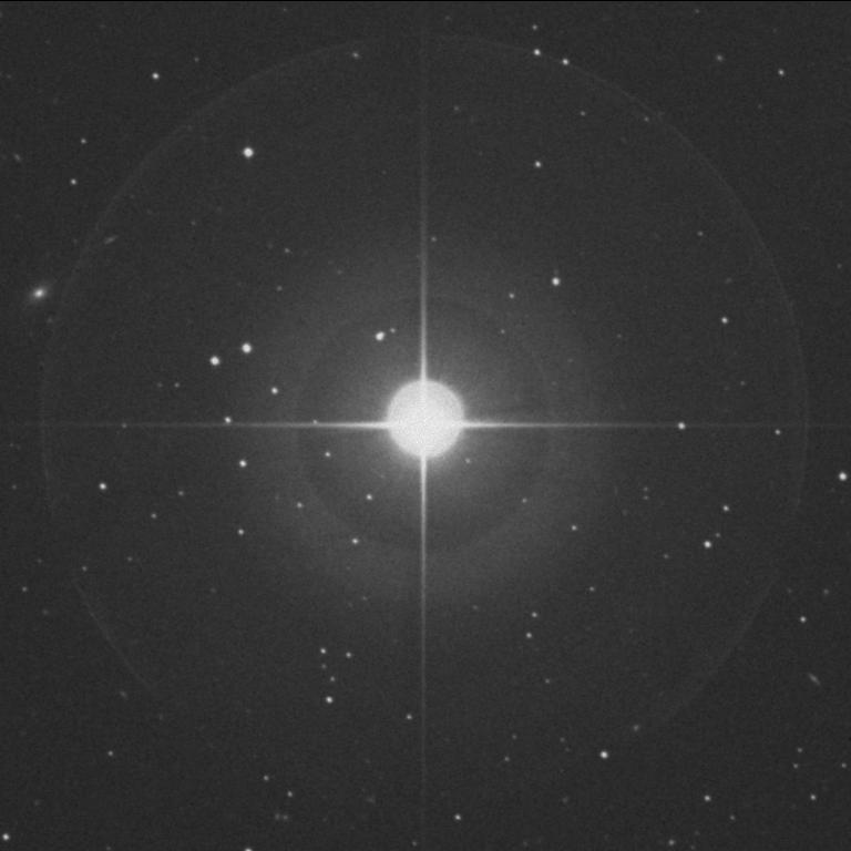
44 Bootis from the Palomar Sky Survey. Image credit: The CDS/Aladin previewer
How good are your optics? Nothing can challenge the resolution of a large light bucket telescope, like attempting to split close double stars. This week, we’d like to highlight a curious triple star system that presents a supreme challenge over the next few years and will ‘keep on giving’ for decades to come.
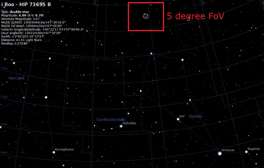
The location of 44 Boötis in the constellation of the Herdsman. Image credit: Stellarium click image to enlarge
The star system in question is 44 Boötis, in the umlaut-adorned constellation of Boötes the herdsman. Boötes is still riding high to the west at dusk for northern hemisphere observers in late August, providing observers a chance to split the pair during prime-time viewing hours.
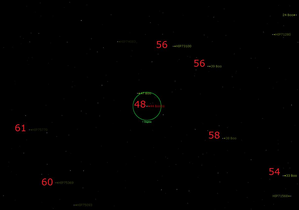
A close up of the five degree wide field of view for 44 Boötis. Note: magnitudes for nearby stars are noted minus decimal points. Image credit: Starry Night Education software.
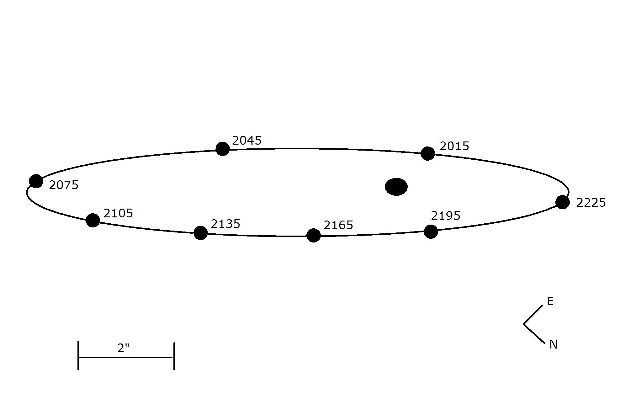
Sometimes also referred to as Iota Boötis, William Herschel first measured the angular separation of the pair in 1781, and F.G.W. Struve discovered the binary nature of 44 Boötis in 1832. Back then, the pair was headed towards a maximum apparent separation of 5 arc seconds in 1870. We call this point apastron. A fast forward to 2015 sees the situation reversed, as the pair currently sits about an arc second apart, and closing. 44 Boötis will pass a periastron of just 0.23” from the primary in 2020. Can you split the pair now? How ‘bout in 2016 onward? Can you recover the split, post 2020?
The apparent orbit of 44 Boötis over the next two centuries. Image credit: Dave Dickinson
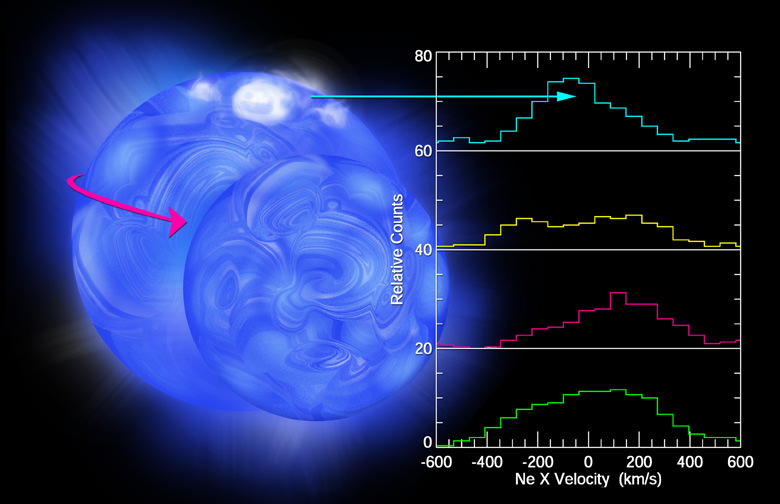
The physical parameters of the system are amazing. About 42 light years distant, 44 Boötis A is 1.05 times as massive as our Sun, and shines at magnitude +4.8. The B component is in a 210 year elliptical orbit with a semi-major axis of 49 AUs (for comparison, Pluto at aphelion is 49 AUs from the Sun), and is itself a curious contact spectroscopic binary about one magnitude fainter. Though you won’t be able to split the B-C pair with a backyard telescope, they betray their presence to professional instruments due to their intertwined spectra. 44 Boötis B and C have a combined mass of 1.5 times that of our Sun, and orbit each other once every 6.4 hours at a center-to-center distance of only 750,000 miles, or only 3 times the distance from Earth to the Moon:
The strange system of 44 Bootis B-C. Note the diameters of the Earth and Moon aren’t to scale. Image credit: Dave Dickinson
That’s close enough that the pair shares a merging atmosphere. It’s a mystery as to just how these types of contact binary stars form, and it would be fascinating to see 44 Boötis up close. This fast spin along our line of sight also means that 44 Boötis B-C varies in brightness by about half a magnitude over a six hour span.
An artist’s conception of the B-C pair of the 44 Boötis system, using data from the Chandra X-ray observatory. Image credit: NASA/CXC/M.Weiss
Though the visual 44 Boötis A-B pair doesn’t quite have an orbital period that the average humanoid could expect to live through, beginning amateur astronomers can watch as the pair once again heads towards a wide an easy 5” split during apastron around 2080.
Collimation, or the near-perfect alignment of optics, is key to the splitting close binaries, and also serves as a good test of a telescope and the stability of the atmosphere. A well-collimated scope will display stars with sharp round Airy disks, looking like luminescent circular ripples in a pond. We call the lower boundary to splitting double stars the Dawes Limit, and on most nights, atmospheric seeing will limit this to about an arc second.
But there’s another method that you can use to ‘split’ doubles closer than an arc second, known as interferometry. This relies on observing the star by use of a filtering mask with two slits that vary in distance across the aperture of the scope. When the mask is rotated to the appropriate position angle and the slits are adjusted properly, the ‘fringes’ of the star snap into focus. A formula utilizing the slit separation can then calculate the separation of the close binary pair. This method works with stars that are A). Closer than 1” separation, and B). Vary by not more than a magnitude in brightness difference.
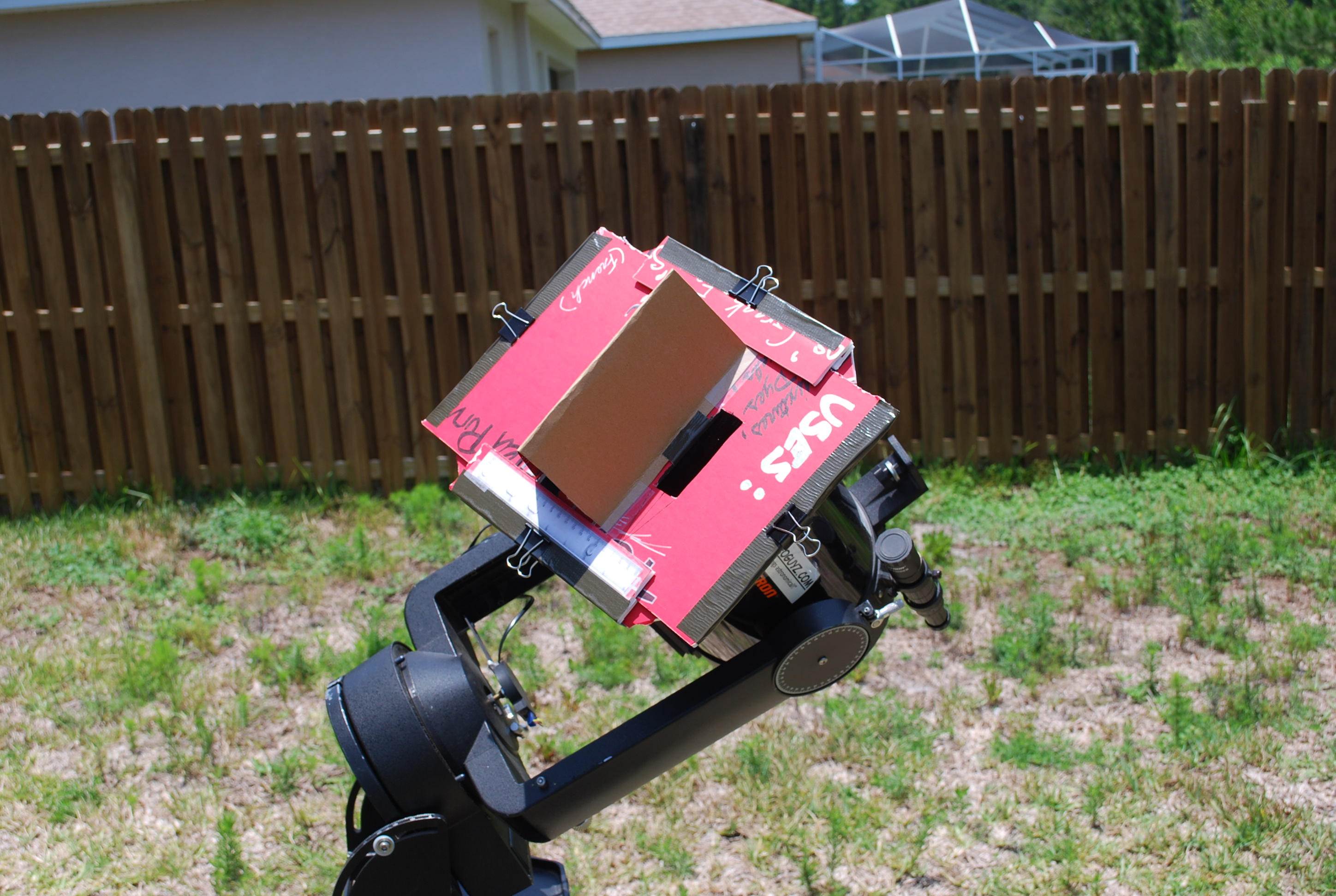
A homemade cardboard interferometer. Image credit: Dave Dickinson
44 Boötis near periastron definitely qualifies. As of this writing, our ‘cardboard interferometer’ is still very much a work in progress. We could envision a more complex version of this rig mechanized, complete with video analysis. Hey, if nothing else, it really draws stares from fellow amateur astronomers…
We promise to delve into the exciting realm of backyard cardboard interferometry once we’ve worked all of the bugs out. In the meantime, be sure to regale us with your tales of tragedy and triumph observing 44 Boötis. Revisiting double stars can pose a life-long pursuit!
– Be sure to check out another double star challenge from Universe Today, with the hunt for Sirius B.
In the 18th century, observations made of all the known planets (Mercury, Venus, Earth, Mars, Jupiter, and Saturn) led astronomers to discern a pattern in their orbits. Eventually, this led to the Titius–Bode Law, which predicted the amount of space between the planets. In accordance with this law, there appeared to be a discernible gap between the orbits of Mars and Jupiter, and investigation into it led to a major discovery.
In addition to several larger objects being observed, astronomers began to notice countless smaller bodies also orbiting between Mars and Jupiter. This led to the creation of the term “asteroid”, as well as “Asteroid Belt” once it became clear just how many there were. Since that time, the term has entered common usage and become a mainstay of our astronomical models.
Discovery:
In 1800, hoping to resolve the issue created by the Titius-Bode Law, astronomer Baron Franz Xaver von Zach recruited 24 of his fellow astronomers into a club known as the “United Astronomical Society” (sometimes referred to the as “Stellar Police”). At the time, its ranks included famed astronomer William Herschel, who had discovered Uranus and its moons in the 1780s.
Ironically, the first astronomer to make a discovery in this regions was Giuseppe Piazzi – the chair of astronomy at the University of Palermo – who had been asked to join the Society but had not yet received the invitation. On January 1st, 1801, Piazzi observed a tiny object in an orbit with the exact radius predicted by the Titius-Bode law.
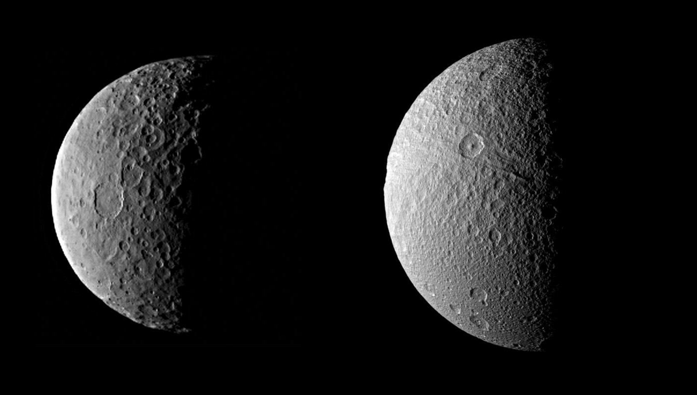
Ceres (left, Dawn image) compared to Tethys (right, Cassini image) at comparative scale sizes. Credits: NASA/JPL-Caltech/UCLA/MPS/DLR/IDA and NASA/JPL-Caltech/SSI. Comparison by J. Major.
Initially, he believed it to be a comet, but ongoing observations showed that it had no coma. This led Piazzi to consider that the object he had found – which he named “Ceres” after the Roman goddess of the harvest and patron of Sicily – could, in fact, be a planet. Fifteen months later, Heinrich Olbers ( a member of the Society) discovered a second object in the same region, which was later named 2 Pallas.
In appearance, these objects seemed indistinguishable from stars. Even under the highest telescope magnifications, they did not resolve into discs. However, their rapid movement was indicative of a shared orbit. Hence, William Herschel suggested that they be placed into a separate category called “asteroids” – Greek for “star-like”.
By 1807, further investigation revealed two new objects in the region, 3 Juno and 4 Vesta; and by 1845, 5 Astraea was found. Shortly thereafter, new objects were found at an accelerating rate, and by the early 1850s, the term “asteroids” gradually came into common use. So too did the term “Asteroid Belt”, though it is unclear who coined that particular term. However, the term “Main Belt” is often used to distinguish it from the Kuiper Belt.
One hundred asteroids had been located by mid-1868, and in 1891 the introduction of astrophotography by Max Wolf accelerated the rate of discovery even further. A total of 1,000 asteroids were found by 1921, 10,000 by 1981, and 100,000 by 2000. Modern asteroid survey systems now use automated means to locate new minor planets in ever-increasing quantities.
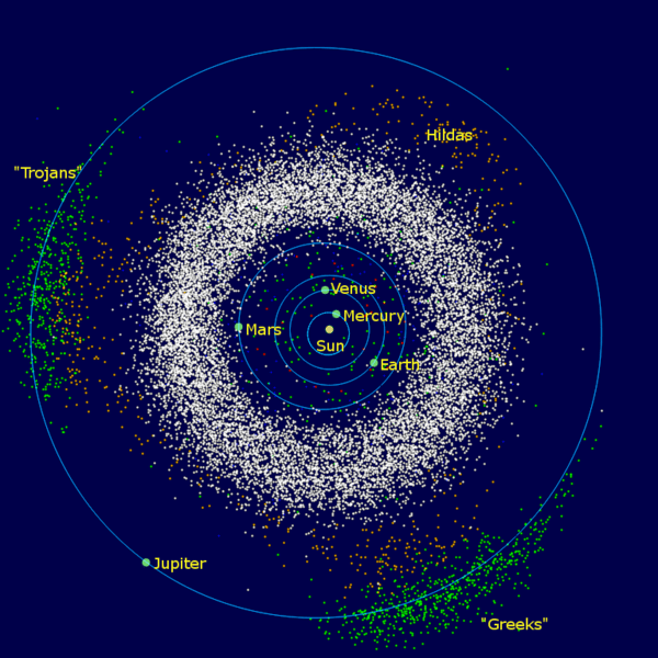
The asteroids of the inner Solar System and Jupiter: The donut-shaped asteroid belt is located between the orbits of Jupiter and Mars. Credit: Wikipedia Commons
Structure:
Despite common perceptions, the Asteroid Belt is mostly empty space, with the asteroids spread over a large volume of space. Nevertheless, hundreds of thousands of asteroids are currently known, and the total number ranges in the millions or more. Over 200 asteroids are known to be larger than 100 km in diameter, and a survey in the infrared wavelengths has shown that the asteroid belt has 0.7–1.7 million asteroids with a diameter of 1 km (0.6 mi) or more.
Located between Mars and Jupiter, the belt ranges from 2.2 to 3.2 astronomical units (AU) from the Sun and is 1 AU thick. Its total mass is estimated to be 2.8×10²¹ to 3.2×10²¹ kilograms – which is equivalent to about 4% of the Moon’s mass. The four largest objects – Ceres, 4 Vesta, 2 Pallas, and 10 Hygiea – account for half of the belt’s total mass, with almost one-third accounted for by Ceres alone.
The main (or core) population of the asteroid belt is sometimes divided into three zones, which are based on what is known as Kirkwood Gaps. Named after Daniel Kirkwood, who announced in 1866 the discovery of gaps in the distance of asteroids, these describe the dimensions of an asteroid’s orbit based on its semi-major axis.
Within this scheme, there are three zones. Zone I lies between the 4:1 resonance and 3:1 resonance Kirkwood gaps, which are 2.06 and 2.5 AU from the Sun respectively. Zone II continues from the end of Zone I out to the 5:2 resonance gap, which is 2.82 AU from the Sun. Zone III extends from the outer edge of Zone II to the 2:1 resonance gap at 3.28 AU.
The asteroid belt may also be divided into the inner and outer belts, with the inner belt formed by asteroids orbiting nearer to Mars than the 3:1 Kirkwood gap (2.5 AU), and the outer belt formed by those asteroids closer to Jupiter’s orbit.
The asteroids that have a radius of 2.06 AU from the Sun can be considered the inner boundary of the asteroid belt. Perturbations by Jupiter send bodies straying there into unstable orbits. Most bodies formed inside the radius of this gap were swept up by Mars (which has an aphelion at 1.67 AU) or ejected by its gravitational perturbations in the early history of the Solar System.
The temperature of the Asteroid Belt varies with the distance from the Sun. For dust particles within the belt, typical temperatures range from 200 K (-73 °C) at 2.2 AU down to 165 K (-108 °C) at 3.2 AU. However, due to rotation, the surface temperature of an asteroid can vary considerably as the sides are alternately exposed to solar radiation and then to the stellar background.
Composition:
Much like the terrestrial planets, most asteroids are composed of silicate rock while a small portion contains metals such as iron and nickel. The remaining asteroids are made up of a mix of these, along with carbon-rich materials. Some of the more distant asteroids tend to contain more ices and volatiles, which includes water ice.
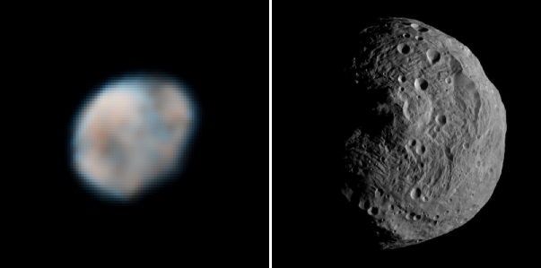
Vesta seen from the Earth-orbit based Hubble Space Telescope in 2007 (left) and up close with the Dawn spacecraft in 2011. Hubble Credit: NASA, ESA, and L. McFadden (University of Maryland). Dawn Credit: NASA/JPL-Caltech/UCLA/MPS/DLR/IDA. Photo Combination: Elizabeth Howell
The Main Belt consists primarily of three categories of asteroids: C-type, or carbonaceous asteroids; S-type, or silicate asteroids; and M-type, or metallic asteroids. Carbonaceous asteroids are carbon-rich, dominate the belt’s outer regions, and comprise over 75% of the visible asteroids. Their surface composition is similar to that of carbonaceous chondrite meteorites while their spectra is similar to what the early Solar System’s is believed to be.
S-type (silicate-rich) asteroids are more common toward the inner region of the belt, within 2.5 AU of the Sun. These are typically composed of silicates and some metals, but not a significant amount of carbonaceous compounds. This indicates that their materials have been modified significantly over time, most likely through melting and reformation.
M-type (metal-rich) asteroids form about 10% of the total population and are composed of iron-nickel and some silicate compounds. Some are believed to have originated from the metallic cores of differentiated asteroids, which were then fragmented from collisions. Within the asteroid belt, the distribution of these types of asteroids peaks at a semi-major axis of about 2.7 AU from the Sun.
There’s also the mysterious and relatively rare V-type (or basaltic) asteroids. This group takes their name from the fact that until 2001, most basaltic bodies in the Asteroid Belt were believed to have originated from the asteroid Vesta. However, the discovery of basaltic asteroids with different chemical compositions suggests a different origin. Current theories of asteroid formation predict that the V-type asteroids should be more plentiful, but 99% of those that have been predicted are currently missing.
Families and Groups:
Approximately one-third of the asteroids in the asteroid belt are members of an asteroid family. These are based on similarities in orbital elements – such as semi-major axis, eccentricity, orbital inclinations, and similar spectral features, all of which indicate a common origin. Most likely, this would have involved collisions between larger objects (with a mean radius of ~10 km) that then broke up into smaller bodies.
This artist’s conception shows how families of asteroids are created. Credit: NASA/JPL-Caltech
Some of the most prominent families in the asteroid belt are the Flora, Eunomia, Koronis, Eos, and Themis families. The Flora family, one of the largest with more than 800 known members, may have formed from a collision less than a billion years ago. Located within the inner region of the Belt, this family is made up of S-type asteroids and accounts for roughly 4-5% of all Belt objects.
The Eunomia family is another large grouping of S-type asteroids, which takes its name from the Greek goddess Eunomia (goddess of law and good order). It is the most prominent family in the intermediate asteroid belt and accounts for 5% of all asteroids.
The Koronis family consists of 300 known asteroids which are thought to have been formed at least two billion years ago by a collision. The largest known, 208 Lacrimosa, is about 41 km (25 mi) in diameter, while an additional 20 more have been found that are larger than 25 km in diameter.
The Eos (or Eoan) family is a prominent family of asteroids that orbit the Sun at a distance of 2.96 – 3.03 AUs, and are believed to have formed from a collision 1-2 billion years ago. It consists of 4,400 known members that resemble the S-type asteroid category. However, the examination of Eos and other family members in the infrared show some differences with the S-type, thus why they have their own category (K-type asteroids).
Asteroids we’ve seen up close show cratered surfaces similar to yet different from much of the cratering on comets. Credit: NASA
The Themis asteroid family is found in the outer portion of the asteroid belt, at a mean distance of 3.13 AU from the Sun. This core group includes the asteroid 24 Themis (for which it is named) and is one of the more populous asteroid families. It is made up of C-type asteroids with a composition believed to be similar to that of carbonaceous chondrites and consists of a well-defined core of larger asteroids and a surrounding region of smaller ones.
The largest asteroid to be a true member of a family is 4 Vesta. The Vesta family is believed to have formed as the result of a crater-forming impact on Vesta. Likewise, the HED meteorites may also have originated from Vesta as a result of this collision.
Along with the asteroid bodies, the asteroid belt also contains bands of dust with particle radii of up to a few hundred micrometers. This fine material is produced, at least in part, from collisions between asteroids, and by the impact of micrometeorites upon the asteroids. Three prominent bands of dust have been found within the asteroid belt – which have similar orbital inclinations as the Eos, Koronis, and Themis asteroid families – and so are possibly associated with those groupings.
Origin:
Originally, the Asteroid Belt was thought to be the remnants of a much larger planet that occupied the region between the orbits of Mars and Jupiter. This theory was originally suggested by Heinrich Olbders to William Herschel as a possible explanation for the existence of Ceres and Pallas. However, this hypothesis has since fallen out of favor for a number of reasons.
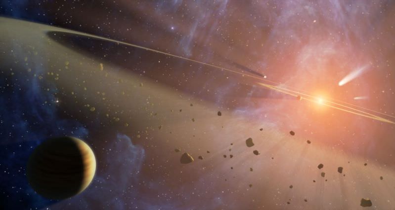
Artist’s impression of the early Solar System, where collisions between particles in an accretion disc led to the formation of planetesimals and eventually planets. Credit: NASA/JPL-Caltech
First, there is the amount of energy it would have required to destroy a planet, which would have been staggering. Second, there is the fact that the entire mass of the Belt is only 4% that of the Moon. Third, the significant chemical differences between the asteroids do not point towards them having been once part of a single planet.
Today, the scientific consensus is that, rather than fragmenting from a progenitor planet, the asteroids are remnants from the early Solar System that never formed a planet at all. During the first few million years of the Solar System’s history, when gravitational accretion led to the formation of the planets, clumps of matter in an accretion disc coalesced to form planetesimals. These, in turn, came together to form planets.
However, within the region of the Asteroid Belt, planetesimals were too strongly perturbed by Jupiter’s gravity to form a planet. These objects would continue to orbit the Sun as before, occasionally colliding and producing smaller fragments and dust.
During the early history of the Solar System, the asteroids also melted to some degree, allowing elements within them to be partially or completely differentiated by mass. However, this period would have been necessarily brief due to their relatively small size, and likely ended about 4.5 billion years ago, in the first tens of millions of years of the Solar System’s formation.
Though they are dated to the early history of the Solar System, the asteroids (as they are today) are not samples of its primordial self. They have undergone considerable evolution since their formation, including internal heating, surface melting from impacts, space weathering from radiation, and bombardment by micrometeorites. Hence, the Asteroid Belt today is believed to contain only a small fraction of the mass of the primordial belt.
Computer simulations suggest that the original asteroid belt may have contained as much mass as Earth. Primarily because of gravitational perturbations, most of the material was ejected from the belt a million years after its formation, leaving behind less than 0.1% of the original mass. Since then, the size distribution of the asteroid belt is believed to have remained relatively stable.
When the asteroid belt was first formed, the temperatures at a distance of 2.7 AU from the Sun formed a “snow line” below the freezing point of water. Essentially, planetesimals formed beyond this radius were able to accumulate ice, some of which may have provided a water source of Earth’s oceans (even more so than comets).
Exploration:
The asteroid belt is so thinly populated that several unmanned spacecraft have been able to move through it; either as part of a long-range mission to the outer Solar System, or (in recent years) as a mission to study larger Asteroid Belt objects. In fact, due to the low density of materials within the Belt, the odds of a probe running into an asteroid are now estimated at less than one in a billion.
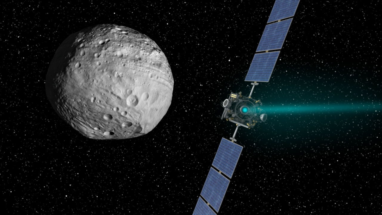
Artist’s concept of the Dawn spacecraft arriving at Vesta. Image credit: NASA/JPL-Caltech
The first spacecraft to make a journey through the asteroid belt was the Pioneer 10 spacecraft, which entered the region on July 16th, 1972. As part of a mission to Jupiter, the craft successfully navigated through the Belt and conducted a flyby of Jupiter (which culminated in December of 1973) before becoming the first spacecraft to achieve escape velocity from the Solar System.
For the most part, these missions were part of missions to the outer Solar System, where opportunities to photograph and study asteroids were brief. Only the Dawn, NEAR and JAXA’s Hayabusamissions have studied asteroids for a protracted period in orbit and at the surface. Dawn explored Vesta from July 2011 to September 2012 and is currently orbiting Ceres (and sending back many interesting pictures of its surface features).
And someday, if all goes well, humanity might even be in a position to begin mining the asteroid belt for resources – such as precious metals, minerals, and volatiles. These resources could be mined from an asteroid and then used in space of in-situ utilization (i.e. turning them into construction materials and rocket propellant), or brought back to Earth.
It is even possible that humanity might one day colonize larger asteroids and establish outposts throughout the Belt. In the meantime, there’s still plenty of exploring left to do, and quite possibly millions of more objects out there to study.
Need an easy way to remember the order of the planets in our Solar System? The technique used most often to remember such a list is a mnemonic device. This uses the first letter of each planet as the first letter of each word in a sentence. Supposedly, experts say, the sillier the sentence, the easier it is to remember.
So by using the first letters of the planets, (Mercury, Venus, Earth, Mars, Jupiter, Saturn, Uranus, and Neptune), create a silly but memorable sentence.
Here are a few examples:
My Very Excellent Mother Just Served Us Noodles (or Nachos)
Mercury’s Volcanoes Erupt Mulberry Jam Sandwiches Until Noon
Very Elderly Men Just Snooze Under Newspapers
My Very Efficient Memory Just Summed Up Nine
My Very Easy Method Just Speeds Up Names
My Very Expensive Malamute Jumped Ship Up North
The Sun and planets to scale. Credit: Illustration by Judy Schmidt, texture maps by Björn Jónsson
If you want to remember the planets in order of size, (Jupiter, Saturn, Uranus, Neptune, Earth, Venus Mars, Mercury) you can create a different sentence:
Just Sit Up Now Each Monday Morning
Jack Sailed Under Neath Every Metal Mooring
Rhymes are also a popular technique, albeit they require memorizing more words. But if you’re a poet (and don’t know it) try this:
Amazing Mercury is closest to the Sun,
Hot, hot Venus is the second one,
Earth comes third: it’s not too hot,
Freezing Mars awaits an astronaut,
Jupiter is bigger than all the rest,
Sixth comes Saturn, its rings look best,
Uranus sideways falls and along with Neptune, they are big gas balls.
Or songs can work too. Here are a couple of videos that use songs to remember the planets:
If sentences, rhymes or songs don’t work for you, perhaps you are more of a visual learner, as some people remember visual cues better than words. Try drawing a picture of the planets in order. You don’t have to be an accomplished artist to do this; you can simply draw different circles for each planet and label each one. Sometimes color-coding can help aid your memory. For example, use red for Mars and blue for Neptune. Whatever you decide, try to pick colors that are radically different to avoid confusing them.
Or try using Solar System flash cards or just pictures of the planets printed on a page (here are some great pictures of the planets). This works well because not only are you recalling the names of the planets but also what they look like. Memory experts say the more senses you involve in learning or storing something, the better you will be at recalling it.
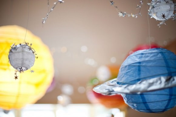
Planets made from paper lanterns. Credit: TheSweetestOccasion.com
Maybe you are a hands-on learner. If so, try building a three-dimensional model of the Solar System. Kids, ask your parents or guardians to help you with this, or parents/guardians, this is a fun project to do with your children. You can buy inexpensive Styrofoam balls at your local craft store to create your model, or use paper lanterns and decorate them. Here are several ideas from Pinterest on building a 3-D Solar System Model.
If you are looking for a group project to help a class of children learn the planets, have a contest to see who comes up with the silliest sentence to remember the planets. Additionally, you can have eight children act as the planets while the rest of the class tries to line them up in order. You can find more ideas on NASA’s resources for Educators. You can use these tricks as a starting point and find more ways of remembering the planets that work for you.
This sequence of images, taken with Rosetta's OSIRIS narrow-angle camera on 30 July 2015, show a boulder-sized object close to the nucleus of Comet 67P/Churyumov-Gerasimenko.
The images were captured on 30 July 2015, about 185 km from the comet. The object measures between one and 50 m across; however, the exact size cannot be determined as it depends on its distance to the spacecraft, which cannot be inferred from these images. Credit: ESA/Rosetta/MPS for OSIRIS Team MPS/UPD/LAM/IAA/SSO/INTA/UPM/DASP/IDA
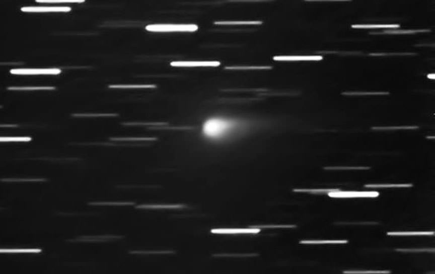
How would you like to see one of the most famous comets with your own eyes? Comet 67P/Churyumov-Gerasimenko plies the morning sky, a little blot of fuzzy light toting an amazing visitor along for the ride — the Rosetta spacecraft. When you look at the coma and realize a human-made machine is buzzing around inside, it seems unbelievable.
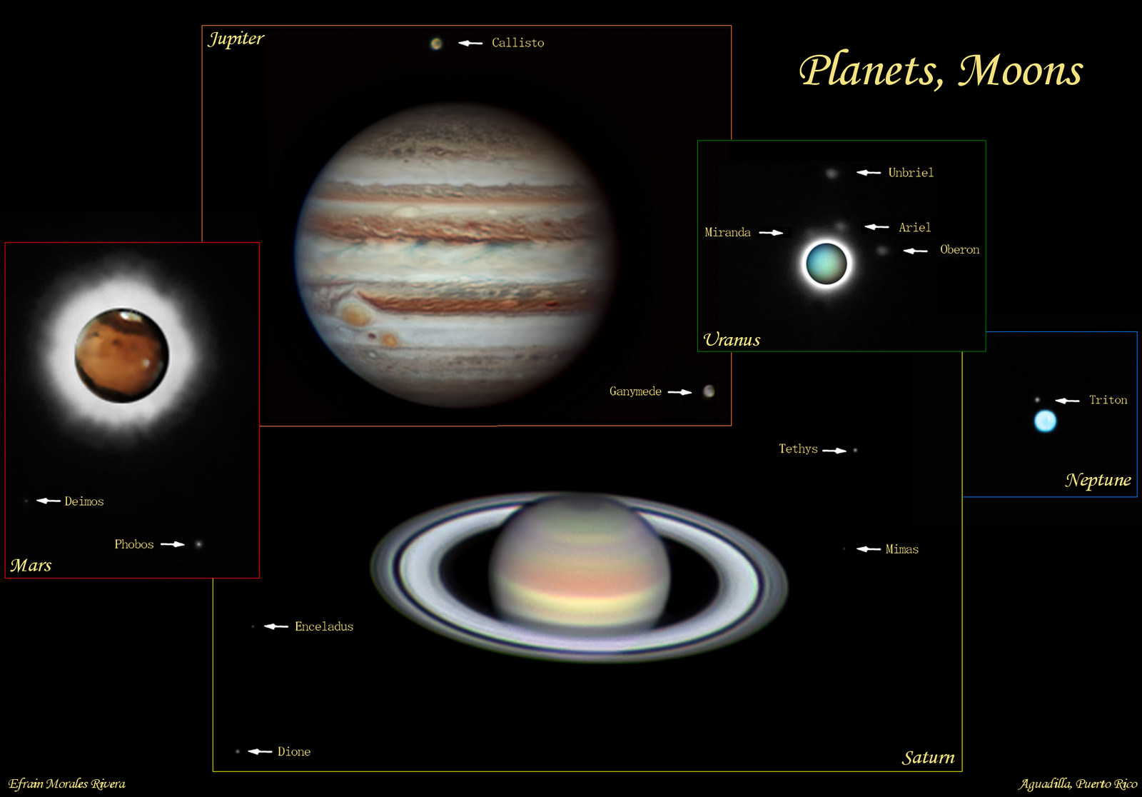
Comet 67P/Churyumov-Gerasimenko plows through a rich star field in Gemini on the morning of August 20, 2015. Photos show a short, faint tail to the west not visible to the eye in most amateur telescopes. Credit: Efrain Morales
If you have a 10-inch or larger telescope, or you’re an experienced amateur with an 8-inch and pristine skies, 67P is within your grasp. The comet glows right around magnitude +12, about as bright as it will get this apparition. Periodic comets generally appear brightest around and shortly after perihelion or closest approach to the Sun, which for 67P/C-G occurred back on August 13.
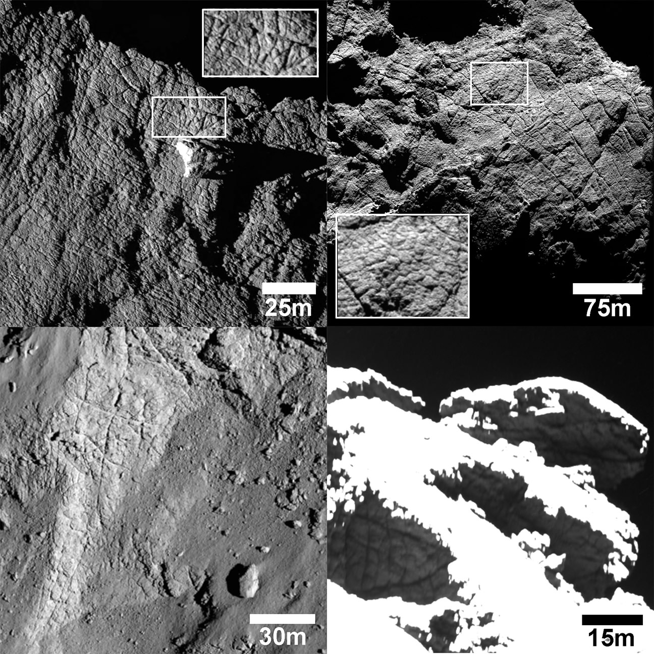
The surface of Comet 67P/C-G is extensively fractured due to loss of volatile ices, the expansion and contraction of the comet from solar heating and bitter cold and possibly even tectonic forces. The smaller polygonal shapes outlined by fractures in the lower right photo are just 6-16 feet (2-5 meters) across. Credit: ESA/Rosetta/MPS for OSIRIS Team MPS/UPD/LAM/IAA/SSO/INTA/UPM/DASP/IDA
You’ll be looking for a small, 1-arc-minute-diameter, compact, circular patch of nebulous light shortly before dawn when it’s highest in the east. Rosetta’s Comet will spend the remainder of August slicing across Gemini the Twins north of an nearly parallel to the ecliptic. I spotted 67P/C-G for the first time this go-round about a week ago in my 15-inch (37 cm) reflector. While it appears like a typical faint comet, thanks to Rosetta, we know this particular rough and tumble mountain of ice better than any previous comet. Photographs show rugged cliffs, numerous cracks due to the expansion and contraction of ice, blowholes that serve as sources for jets and smooth plains blanketed in fallen dust.
Geysers of dust and gas shooting off the comet’s nucleus are called jets. The material they deliver outside the nucleus builds the comet’s coma. Credit: ESA/Rostta/NAVCAM
The jets are geyser-like sprays of dust and gas that loft grit and rocks from the comet’s interior and surface into space to create a coma or temporary atmosphere. This is what you’ll see in your telescope. And if you’re patient, you’ll even be able to catch this glowing tadpole on the move. I was surprised at its speed. After just 20 minutes, thanks to numerous field stars that acted as references, I could easily spot the comet’s eastward movement using a magnification of 245x.
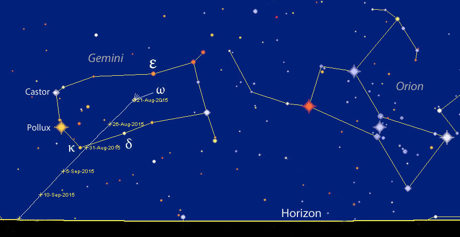
Facing east around 4 a.m. local time in late August, you’ll see the winter constellations Gemini and Orion. 67P/C-G’s path is shown through early September. Brighter stars near the path are labeled. Time shown is 4 a.m. CDT. Use this map to get oriented and then switch to the one below for telescope use. Source: Chris Marriott’s SkyMap
Tomorrow morning, 67P/C-G passes very close to the magnitude +5 star Omega Geminorum. While this will make it easy to locate, the glare may swamp the comet. Set your alarm for an hour before dawn’s start to allow time to set up a telescope, dark-adapt your eyes and track down the field where the comet will be that morning using low magnification.
Once you’ve centered 67P/C-G’s position, increase the power to around 100x-150x and use averted vision to look for a soft, fuzzy patch of light. If you see nothing, take it to the next level (around 200-250x) and carefully search the area. The higher the magnification, the darker the field of view and easier it will be to spot it.
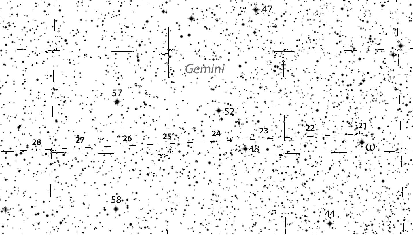
Detailed map showing the comet’s path through central Gemini daily August 21-28, 2015 around 4 a.m. CDT. Brighter stars are marked with Greek letters and numbers. “57”= 57 Geminorum. North is up, east to the left and stars to magnitude +13.5. Click for a larger version you can print out. Source: Chris Marriott’s SkyMap
Besides being relatively faint, the comet doesn’t get very high in the east before the onset of twilight. Low altitude means the atmosphere absorbs a share of the comet’s light, making it appear even fainter. Not that I want to dissuade you from looking! There’s nothing like seeing real 67P photons not to mention the adventure and sense of accomplishment that come from finding the object on your own.
As we advance into late summer and early fall, 67P/C-G will appear higher up but also be fading. Now through about August 27 and again from September 10-24 will be your best viewing times. That’s when the Moon’s absent from the sky.
Given the comet’s current distance from Earth of 165 million miles and apparent visual size of just shy of 1 arc minute, the coma measures very approximately 30,000 miles across. Rosetta orbits the comet’s 2.5-mile-long icy nucleus at a distance of about 115 miles (186 km), meaning it’s snug up against the nuclear center from our point of view on the ground.
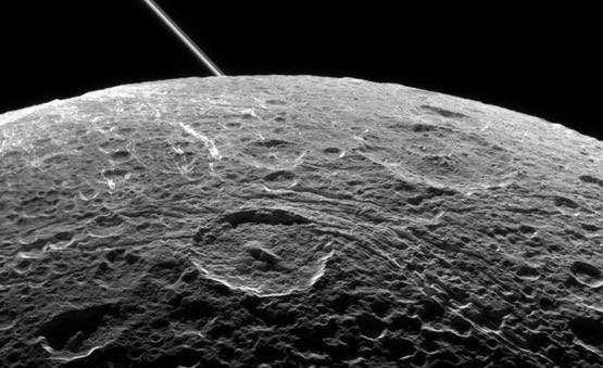
NASA’s Cassini spacecraft paid a visit to Saturn’s moon Dione this week, one final time.
Cassini passed just 474 kilometers (295 miles) above the surface of the icy moon on Monday, August 17th at 2:33 PM EDT/18:33 UT. The flyby is the fifth and final pass of Cassini near Dione (pronounced dahy-OH-nee). The closest passage was 100 kilometers (60 miles) in December 2011. This final flyby of Dione will give researchers a chance to probe the tiny world’s internal structure, as Cassini flies through the gravitational influence of the moon. Cassini has only gathered gravity science data on a handful of Saturn’s 62 known moons.
“Dione has been an enigma, giving hints of active geologic processes, including a transient atmosphere and evidence of ice volcanoes. But we’ve never found the smoking gun,” said Cassini science team member Bonnie Buratti in a recent press release. “The fifth flyby of Dione will be the last chance.”
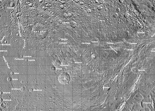
A map of Dione. Click here for a full large .pdf map. Credit: USGS
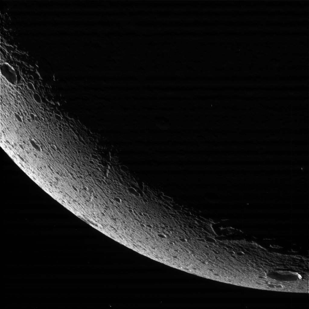
Voyager 1 gave us our very first look at Dione in 1980, and Cassini has explored the moon in breathtaking detail since its first flyby in 2005. This final pass targeted Dione’s north pole at a resolution of only a few meters. Cassini’s Infrared Spectrometer was also on the lookout for any thermal anomalies, a good sign that Dione may still be geologically active. The spacecraft’s Cosmic Dust Analyzer also carried out a search for any dust particles coming from Dione. The results of these experiments are forthcoming. In a synchronous rotation, Dione famously displays a brighter leading hemisphere, which has been pelted with E Ring deposits.
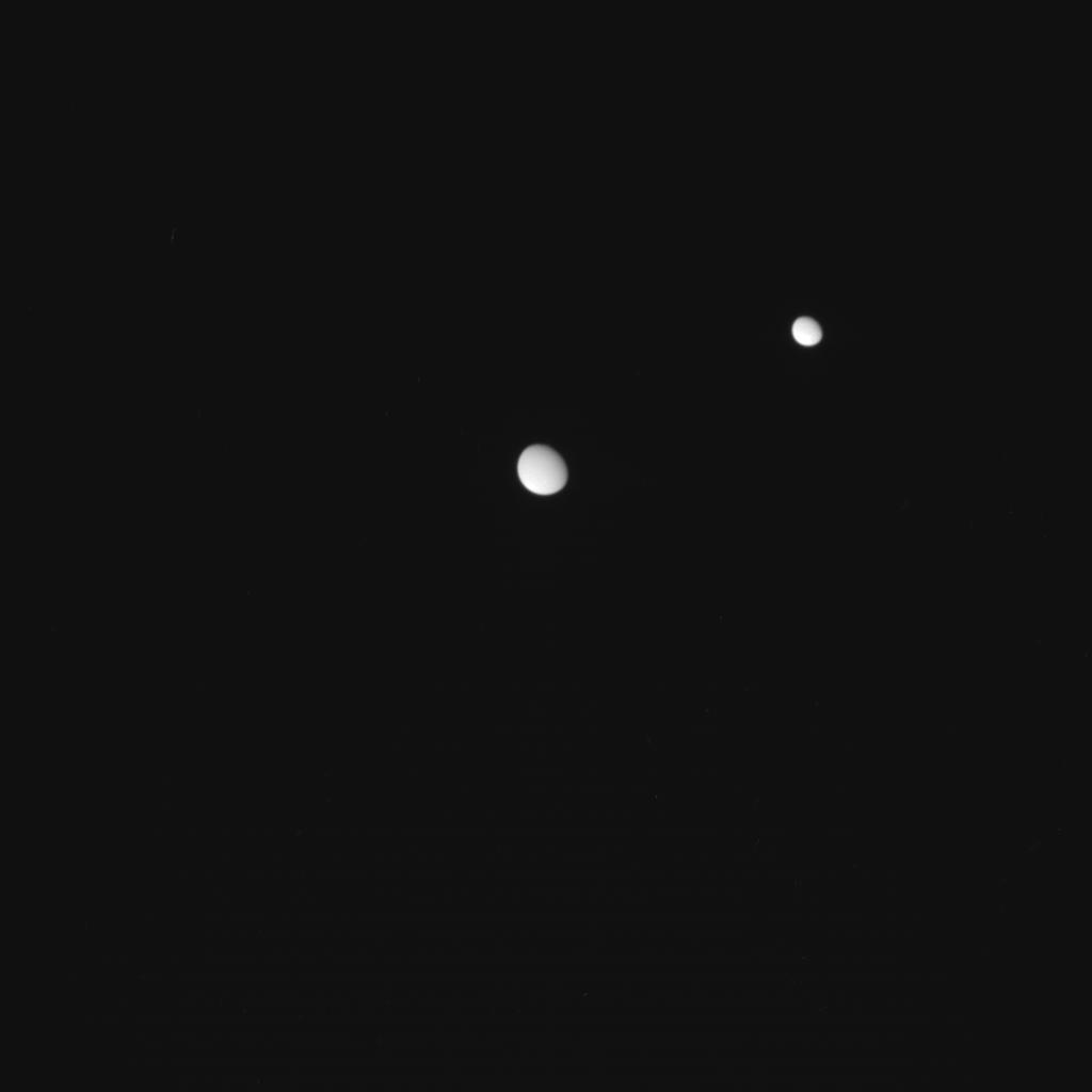
Dione (center) with Enceladus(smaller and to the upper right) in the distance. Image credit: NASA/JPL-Caltech/Space Science Institute
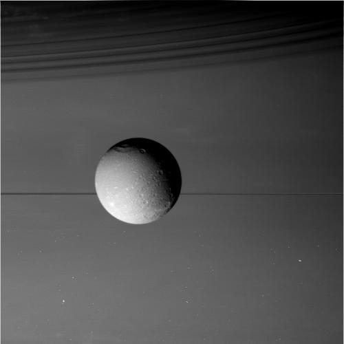
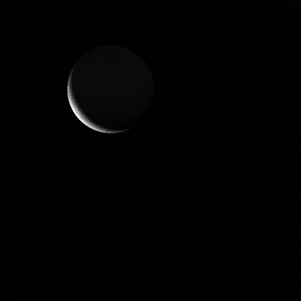
The raw images from this week’s flyby are now available on the NASA Cassini website. You can see the sequence of the approach, complete with a ‘photobomb’ of Saturn’s moon Enceladus early on. Dione then makes a majestic pass in front of Saturn’s rings and across the ochre disk of the planet itself, before snapping into dramatic focus. Here we see the enormous shattered Evander impact basin near the pole of Dione, along with Erulus crater with a prominent central peak right along the day/night terminator. Dione has obviously had a battered and troubled past, one that astro-geologists are still working out. Cassini then takes one last shot, giving humanity a fitting final look at Dione as a crescent receding off in the distance.
Dione in profile against Saturn. Image credit: NASA/JPL-Caltech/Space Science Institute
It’ll be a long time before we visit Dione again.
“This will be our last chance to see Dione up close for many years to come,” said Cassini mission deputy project scientist Scott Edgington. “Cassini has provided insights into this icy moon’s mysteries, along with a rich data set and a host of new questions for scientists to ponder.”
Cassini also took a distant look at Saturn’s tiny moon Hyrrokkin (named after the Norse giantess who launched Baldur’s funeral ship) earlier this month. Though not a photogenic pass, looking at the tinier moons of Saturn helps researchers better understand and characterize their orbits. Even after more than a decade at Saturn, there are tiny moons of Saturn that Cassini has yet to see up close.
The limb of Dione on close approach. Image credit: NASA/JPL-Caltech/Space Science Institute
Next up for Cassini is a pass 1,036 kilometers (644 miles) from the surface of Titan on September 28th, 2015.
Launched in 1997, Cassini has given us over a decade’s worth of exploration of the Saturnian system, including the delivery of the European Space Agency’s Huygens lander to the surface of Titan. The massive moon may be the target of a proposed mission that could one day sail the hazy atmosphere of Titan, complete with a nuclear plutonium powered MMRTG and deployable robotic quadcopters.
Cassini is set to depart the equatorial plane of Saturn late this year, for a series of maneuvers that will feature some dramatic passes through the rings before a final fiery reentry into the atmosphere of Saturn in 2017.
A farewell look at Dione. Image credit: NASA/JPL-Caltech/Space Science Institute
Astronomer Giovanni Cassini discovered Dione on March 21st, 1684 from the Paris observatory using one of his large aerial refracting telescopes. About 1,120 kilometers in diameter, Dione is 1.5% as massive as Earth’s Moon. Dione orbits Saturn once every 2.7 days, and is in a 1:2 resonance with Enceladus, meaning Dione completes one orbit for every two orbits of Enceladus.
In a backyard telescope, Dione is easily apparent along with the major moons of Saturn as a +10.4 magnitude ‘star.’ Saturn is currently a fine telescopic target in the evening low to the south on the Libra-Scorpius border, offering prime time observers a chance to check out the ringed planet and its moons. Fare thee well, Dione… for now.