Phew! Our eyes and thoughts have been cast so far out into the outer reaches of the solar system following New Horizons and Pluto this week, that we’re just now getting to the astronomical action going on in our own backyard.
New Horizons Flight Controllers celebrate after they received confirmation from the spacecraft that it had successfully completed the flyby of Pluto, Tuesday, July 14, 2015 in the Mission Operations Center (MOC) of the Johns Hopkins University Applied Physics Laboratory (APL), Laurel, Maryland. Credit: NASA/Bill Ingalls
Watch Pluto grow in this series of photos taken during New Horizons’ approach
Whew! We’re out of the woods. On schedule at 9 p.m. EDT, New Horizons phoned home telling the mission team and the rest of the on-edge world that all went well. The preprogrammed “phone call” — a 15-minute series of status messages beamed back to mission operations at the Johns Hopkins University Applied Physics Laboratoryin Maryland through NASA’s Deep Space Network — ended a tense 21-hour waiting period.
The team deliberately suspended communications with New Horizons until it was beyond the Pluto system, so the spacecraft could focus solely on data gathering. With a mountain of information now queued up, it’s estimated it will take 16 months to get it all back home. As the precious morsels arrive bit by byte, New Horizons will sail deeper into the Kuiper Belt looking for new targets until it ultimately departs the Solar System.
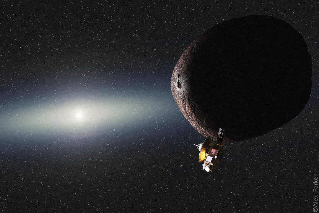
After Pluto, NASA hopes to send New Horizons to another asteroid or two in the Kuiper Belt to perform a flyby and reconnaissance similar to the Pluto mission. Credit: Alex Parker / SwRI
Assuming NASA funds a continuing mission, the team hopes to direct the spacecraft to one or two additional Kuiper Belt objects (KBO) over the next five to seven years. There are presently three possible targets – PT1, PT2, and PT3. (PT = potential target). PT1, imaged by the Hubble Space Telescope, looks like the best option at the moment and could by reached by January 2019. If you thought Pluto was small, PT 1 is only about 25 miles (40 km) across. Much lies ahead.
The image at left shows a KBO at an estimated distance of approximately 4 billion miles from Earth. Its position noticeably shifts between exposures taken approximately 10 minutes apart. The image at right shows a second KBO at roughly a similar distance. Credit: NASA, ESA, SwRI, JHU/APL, and the New Horizons KBO Search Team
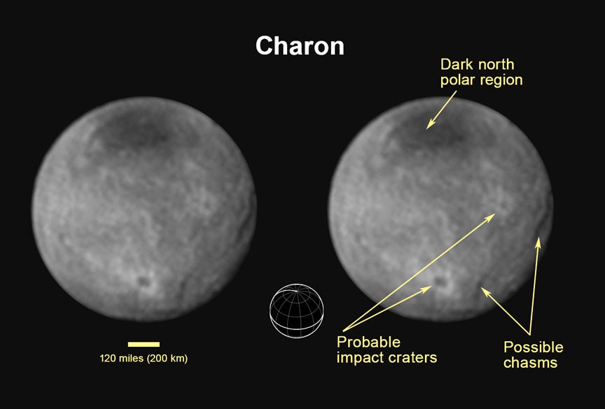
Chasms, craters, and a dark north polar region are revealed in this image of Pluto’s largest moon Charon taken by New Horizons on July 11, 2015. The annotated version includes a diagram showing Charon’s north pole, equator, and central meridian, with the features highlighted. Credits: NASA/JHUAPL/SWRI
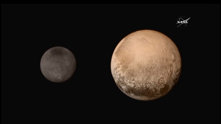
Beginning in 1978, astronomers began to discover that Pluto – the most distant known object from the Sun (at the time) – had its own moons. What had once been thought to be a solitary body occupying the outer edge of our Solar System suddenly appeared to have a system with a large moon Charon. And as time went on, a total of four moons would be discovered.
Of these, Charon is the largest and most easily observed, hence why it was discovered first. In addition to being the biggest of its peers, its also quite large in comparison to Pluto. As such, Charon has always had something of a unique relationship with its parent body, and stands apart as far as objects in the outer Solar System are concerned.
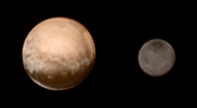
Artist's impression of Charon (left) and Pluto (right), showing their relative sizes. Credit:
‘Here be Dragons…’ read the inscriptions of old maps used by early seafaring explorers. Such maps were crude, and often wildly inaccurate.
The same could be said for our very understanding of distant planetary surfaces today. But this week, we’ll be filling in one of those ‘terra incognita’ labels, as New Horizons conducts humanity’s very first reconnaissance of Pluto and its moons.
The closest approach for New Horizons is set for Tuesday, July 14th at 11:49 UT/7:49 AM EDT, as the intrepid spacecraft passes 12,600 kilometres (7,800 miles) from Pluto’s surface. At over 4 light hours or nearly 32 astronomical units (AUs) away, New Horizons is on its own, and must perform its complex pirouette through the Pluto system as it cruises by at over 14 kilometres (8 miles) a second.
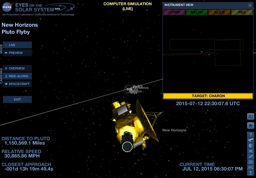
This also means that we’ll be hearing relatively little from the spacecraft on flyby day, as it can’t waste precious time pointing its main dish back at the Earth. With a downlink rate of 2 kilobits a second—think ye ole 1990’s dial-up, plus frozen molasses—it’ll take months to finish off data retrieval post flyby. A great place to watch a simulation of the flyby ‘live’ is JPL’s Eyes on the Solar System, along with who is talking to New Horizons currently on the Deep Space Network with DSN Now.
A snapshot of the current July 13th view of New Horizons as it nears Pluto. (Image credit: NASA’s Eyes on the Solar System).
Bob King also wrote up an excellent timeline of New Horizons events for Universe Today yesterday. Also be sure to check out the Planetary Society’s in-depth look at what to expect by Emily Lakdawalla.
Seems strange that after more than a decade of recycling the same blurry images and artist’s conceptions in articles, we’re now getting a new and improved shot of Pluto and Charon daily!
To follow the tale of Pluto is to know the story of modern planetary astronomy. Discovered in 1930 by American astronomer Clyde Tombaugh from the Lowell Observatory, Pluto was named by 11-year old Venetia Burney. Venetia just passed away in 2009, and there’s a great short documentary interview with her entitled Naming Pluto.
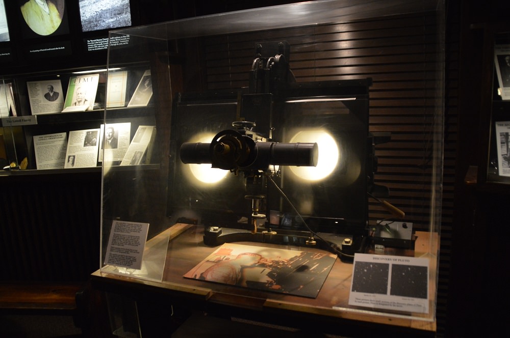
The blink comparitor Clyde Tombaugh used to discover Pluto, on display at the Lowell Observatory. Image Credit: David Dickinson
Fun fact: Historians at the Carnegie Institute recently found images of Pluto on glass plates… dated 1925, from five years before its discovery.
Despite the pop culture reference, Pluto was not named after the Disney dog, but after the Roman god of the underworld. Pluto the dog was not named in Disney features until late 1930, and if anything, the character was more than likely named after the buzz surrounding the newest planet on the block.
We’re already seeing features on Pluto and Charon in the latest images, such as the ‘heart,’ ‘donut,’ and the ‘whale’ of Pluto, along with chasms, craters and a dark patch on Charon. The conspicuous lack of large craters on Pluto suggests an active world.
The International Astronomical Union (IAU) convention for naming any new moons discovered in the Plutonian system specifies characters related to the Roman god Pluto and tales of the underworld.
Brake for New Horizons on July 14th… Image credit: David Dickinson
With features, however, cartographers of Pluto should get a bit more flexibility. Earlier this year, the Our Pluto campaign invited the public to cast votes to name features on Pluto and Charon related to famous scientists, explorers and more. The themes of ‘fictional explorers and vessels’ has, of course, garnered much public interest, and Star Trek’s Mr. Spock and the Firefly vessel Serenity may yet be memorialized on Charon. Certainly, it would be a fitting tribute to the late Leonard Nimoy. We’d like to see Clyde Tombaugh and Venetia Burney paid homage to on Pluto as well.
We’ve even proposed the discovery of a new moon be named after the mythological underworld character Alecto, complete with a Greek ‘ct’ spelling to honor Clyde Tombaugh.
The discovery and naming of Charon in 1978 by astronomer Robert Christy set a similar precedent. Christy choose the name of the mythological boatman who plied the river Styx (which also later became a Plutonian moon) as it included his wife Charlene’s nickname ‘Char.’ This shibboleth also set up a minor modern controversy as to the exact pronunciation of Charon, as the mythological character is pronounced with a hard ‘k’ sound, but most folks (including NASA) say the moon as ‘Sharon’ in keeping with Christy’s in-joke that slipped past the IAU.
And speaking of Pluto’s large moon, someone did rise to the occasion and take our ‘Charon challenge,’ we posed during the ongoing Pluto opposition season recently. Check out this amazing capture of the +17th magnitude moon winking in and out of view next to Pluto courtesy of Wendy Clark:
Click here to see the animation of the possible capture of Charon near Pluto. Image credit and copyright: Wendy Clark
Clark used the 17” iTelescope astrograph located at Siding Spring Observatory in Australia to tease out the possible capture of the itinerant moon.
Great job!
What’s in a name? What strange and wonderful discoveries await New Horizons this week? We should get our very first signal back tomorrow night, as New Horizons ‘phones home’ with its message that it survived the journey around 9:10 PM EDT/1:10 UT. Expect this following Wednesday—in the words of New Horizons principal Investigator Alan Stern—to begin “raining data,” as the phase of interpreting and evaluating information begins.
The women who power the New Horizons mission to Pluto. Image credit: SwRI/JHUAPL
And there’s more in store, as the New Horizons team will make the decision to maneuver the spacecraft for a rendezvous with a Kuiper Belt Object (KBO) next month. Said KBO flyby will occur in the 2019-2020 timeframe, and perhaps, we’ll one day see a Pluto orbiter mission or lander in the decades to come…
Maybe one way journeys to ‘the other Red Planet’ are the wave of the future.’ Pluto One anyone?
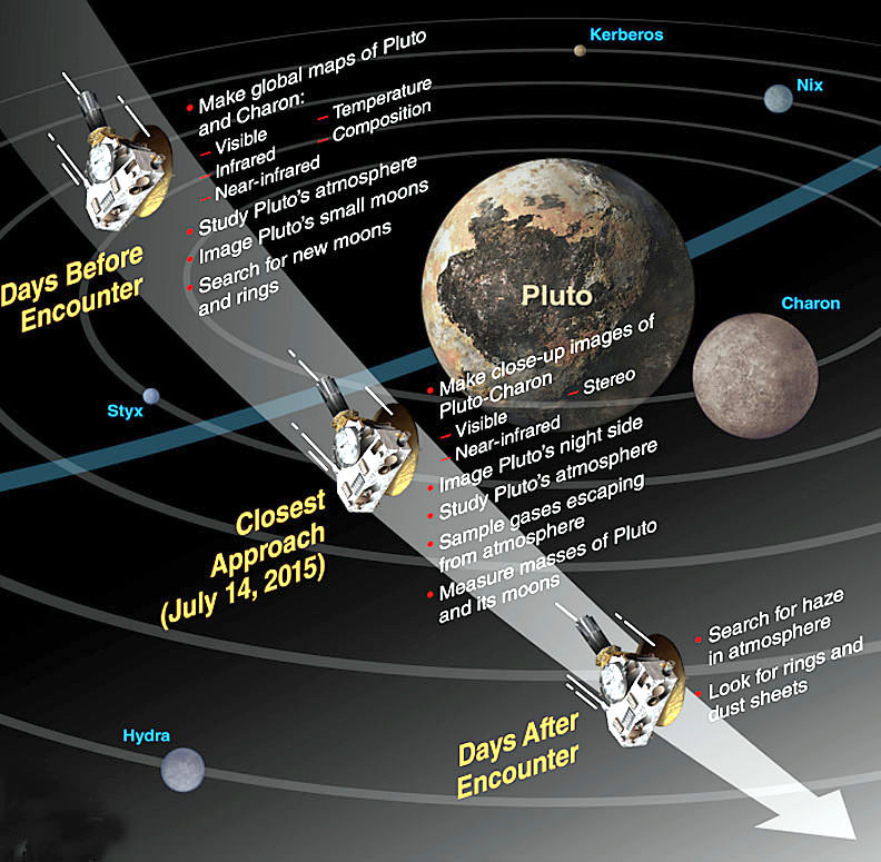
Graphic showing New Horizons' busy schedule before and during the flyby. Credit: NASA
Countdown to discovery! Not since Voyager 2’s flyby of Neptune in 1989 have we flung a probe into the frozen outskirts of the Solar System. Speeding along at 30,800 miles per hour New Horizons will pierce the Pluto system like a smartly aimed arrow.
Newest view of Pluto seen from New Horizons on July 11, 2015 shows a world that continues to grow more fascinating and look stranger every day. See annotated version below. Credits: NASA/JHUAPL/SWRIFor the first time on Pluto, this view reveals linear features that may be cliffs, as well as a circular feature that could be an impact crater. Rotating into view is the bright heart-shaped feature that will be seen in more detail during New Horizons’ closest approach on July 14. The annotated version includes a diagram indicating Pluto’s north pole, equator, and central meridian. Credits: NASA/JHUAPL/SWRI
Edging within 7,800 miles of its surface at 7:49 a.m. EDT, the spacecraft’s long-range telescopic camera will resolve features as small as 230 feet (70 meters). Fourteen minutes later, it will zip within 17,930 miles of Charon as well as image Pluto’s four smaller satellites — Hydra, Styx, Nix and Kerberos.
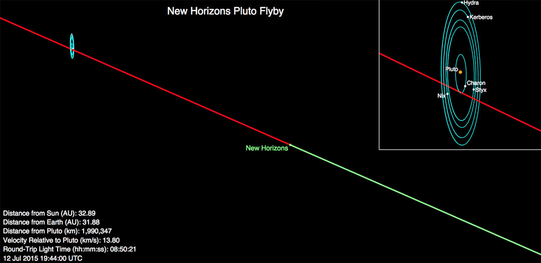
This image shows New Horizons’ current position (3 p.m. EDT July 12) along its planned Pluto flyby trajectory. The green segment of the line shows where New Horizons has traveled; the red indicates the spacecraft’s future path. The Pluto system is tilted on end because the planet’s axis is tipped 123° to the plane of its orbit. Credit: NASA/JHUAPL/SWRI
After zooming past, the craft will turn to photograph Pluto eclipsing the Sun as it looks for the faint glow of rings or dust sheets illuminated by backlight. At the same time, sunlight reflecting off Charon will faintly illuminate Pluto’s backside. What could be more romantic than Charonshine?
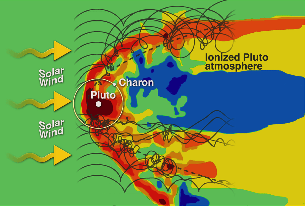
Six other science instruments will build thermal maps of the Pluto-Charon pair, measure the composition of the surface and atmosphere and observe Pluto’s interaction with the solar wind. All of this will happen autopilot. It has to. There’s just no time to send a change instructions because of the nearly 9-hour lag in round-trip communications between Earth and probe.
Instruments New Horizons will use to characterize Pluto are REX (atmospheric composition and temperature); PEPSSI (composition of plasma escaping Pluto’s atmosphere); SWAP (solar wind studies); LORRI (close up camera for mapping, geological data); Star Dust Counter (student experiment measuring space dust during the voyage); Ralph (visible and IR imager/spectrometer for surface composition and thermal maps) and Alice (composition of atmosphere and search for atmosphere around Charon). Credit: NASA/Johns Hopkins University Applied Physics Laboratory/Southwest Research Institute
Want to go along for the ride? Download and install NASA’s interactive app Eyes on Pluto and then click the launch button on the website. You’ll be shown several options including a live view and preview. Click preview and sit back to watch the next few days of the mission unfold before your eyes.
American astronomer Clyde Tombaugh discovered Pluto in 1930 from Lowell Observatory. Tombaugh died in 1997, but an ounce of his ashes, affixed to the spacecraft in a 2-inch aluminum container. “Interned herein are remains of American Clyde W. Tombaugh, discoverer of Pluto and the solar system’s ‘third zone.’ Adelle and Muron’s boy, Patricia’s husband, Annette and Alden’s father, astronomer, teacher, punster, and friend: Clyde Tombaugh (1906-1997)”
Like me, you’ve probably wondered how daylight on Pluto compares to that on Earth. From 3 billion miles away, the Sun’s too small to see as a disk with the naked eye but still wildly bright. With NASA’s Pluto Time, select your city on an interactive mapand get the time of day when the two are equal. For my city, daylight on Pluto equals the gentle light of early evening twilight six minutes after sunset. An ideal time for walking, but step lightly. In Pluto’s gentle gravity, you only weigh 1/15 as much as on Earth.
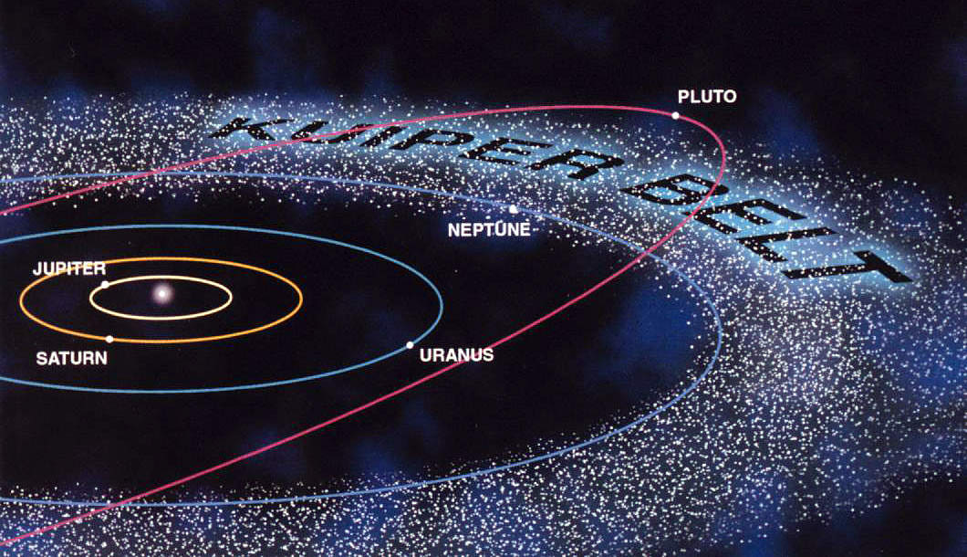
Pluto and its inclined orbit are highlighted among the hundreds of thousands of icy asteroids in the Kuiper Belt beyond Neptune. Credit: NASA
New Horizons is the first mission to the Kuiper Belt, a gigantic zone of icy bodies and mysterious small objects orbiting beyond Neptune. This region also is known as the “third” zone of our solar system, beyond the inner rocky planets and outer gas giants. Pluto is its most famous member, though not necessarily the largest. Eris, first observed in 2003, is nearly identical in size. It’s estimated there are hundreds of thousands of icy asteroids larger than 61 miles (100 km) across along with a trillion comets in the Belt, which begins at 30 a.u. (30 times Earth’s distance from the Sun) and reaches to 55 a.u.
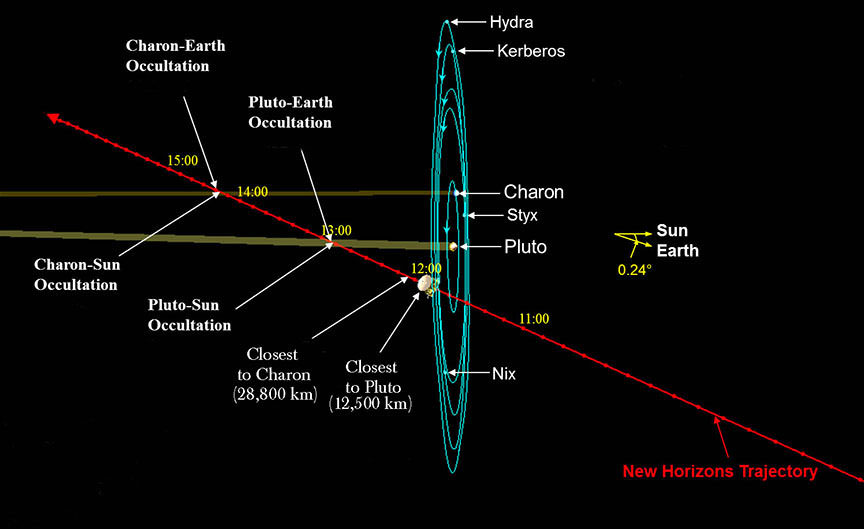
During its fleeting flyby, New Horizons will slice across the Pluto system, turning this way and that to photograph and gather data on everything it can. Crucial occultations are shown that will be used to determine the structure and composition of Pluto’s (and possibly Charon’s) atmosphere. Sunlight reflected from Charon will also faintly illuminate Pluto’s backside. Credit: NASA with additions by the author
Below you’ll find a schedule of events in Eastern Time. (Subtract one hour for Central, 2 hours for Mountain and 3 hours for Pacific). Keep in mind the probe will be busy shooting photos and gathering data during the flyby, so we’ll have to wait until Wednesday July 15 to see the the detailed close ups of Pluto and its moons. Even then, New Horizons’ recorders will be so jammed with data and images, it’ll take months to beam it all back to Earth.
A new photo of Charon, too! Chasms, craters, and a dark north polar region are revealed in this image of Pluto’s largest moon taken by New Horizons on July 11, 2015. The annotated version includes a diagram showing Charon’s north pole, equator, and central meridian, with the features highlighted. The prominent crater is about 60 miles (96 km) across; the chasms appear to be geological faults. Credits: NASA/JHUAPL/SWRI
Fasten your seat belts — we’re in for an exciting ride.
We’ll be reporting on results and sharing photos from the flyby here at Universe Today, but you’ll also want to check out NASA’s live coverage on NASA TV, its website and social media.
Monday, July 13
10:30 a.m. to noon – Media briefing on mission status and what to expect broadcast live on NASA TV
Tuesday, July 14
7:30 to 8 a.m. – Arrival at Pluto! Countdown program on NASA TV
At approximately 7:49 a.m., New Horizons is scheduled to be as close as the spacecraft will get to Pluto, approximately 7,800 miles (12,500 km) above the surface, after a journey of more than 9 years and 3 billion miles. For much of the day, New Horizons will be out of communication with mission control as it gathers data about Pluto and its moons.
The moment of closest approach will be marked during a live NASA TV broadcast that includes a countdown and discussion of what’s expected next as New Horizons makes its way past Pluto and potentially dangerous debris.
8 to 9 a.m. – Media briefing, image release on NASA TV
Wednesday, July 15
3 to 4 p.m. – Media Briefing: Seeing Pluto in a New Light; live on NASA TV and release of close-up images of Pluto’s surface and moons, along with initial science team reactions.
We’ll have the latest Pluto photos for you, but you can also check these excellent sites:
An artist's illustration of Pluto. Credit: NASA/New Horizons
First discovered in 1930, Pluto was considered to be the ninth planet in our Solar System for many decades. And though its status has since been downgraded to that of a dwarf planet, thanks to the discovery of Eris in 2004, Pluto continues to fascinate and intrigue astronomers.
And with the New Horizons mission fast approaching the planet, astronomers are eagerly anticipating the return of photographs and data that will help them answer some burning questions they have about this celestial body – not the least of which is whether or not it supports life!
Surface Conditions:
To be fair, there is virtually no chance that Pluto has life living on its surface. For starters, it orbits our Sun at extreme distances, ranging from 29.657 AU (4,437,000,000 km) at perihelion to 48.871 AU (7,311,000,000 km) at aphelion. At this distance, surface temperatures can reach as low as 33 K (-240 °C or -400 °F).
Not only does water freeze solid at these temperatures, but other liquids and gases that are present on Pluto’s surface – such as methane (CH4), nitrogen gas (N²), and carbon monoxide (CO) – also freeze solid. These compounds have much lower freezing points than water, and so the chance of life surviving under these conditions is slim to nil.
An artist’s concept of frosty Pluto. Credit: ESO/ L. Calçada
And while Pluto has a thin atmosphere, it consists mainly of nitrogen gas, methane and carbon monoxide, which exist in equilibrium with their ices on the surface. At the same time, the surface pressure ranges from s from 6.5 to 24 ?bar (0.65 to 2.4 Pa), which is roughly one million to 100,000 times less than Earth’s atmospheric pressure.
This atmosphere also undergoes transitions as Pluto gets closer and farther away from the Sun. Basically, when Pluto is at perihelion, the atmosphere freezes solid; when it is at aphelion, the surface temperature increases, causing the ices to sublimate.
As such, there is simply no way life could survive on the surface of Pluto. Between the extreme cold, low atmospheric pressure, and constant changes in the atmosphere, no known organism could survive. However, that does not rule out the possibility of life being found inside the planet.
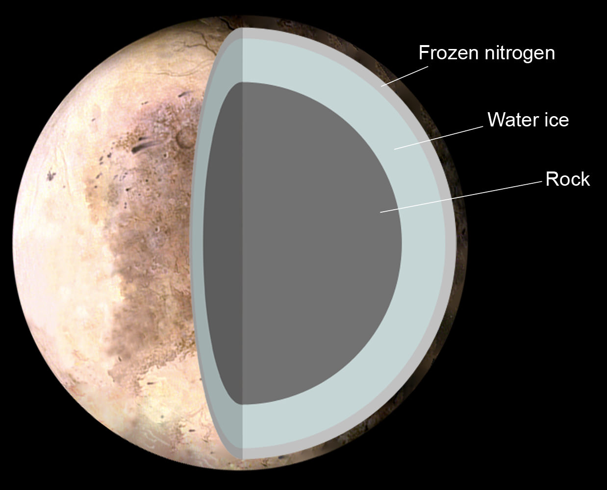
Interior: Like many moons and smaller planetoids in the Outer Solar System, scientists believe that Pluto’s internal structure is differentiated, with rocky material having settled into a dense core surrounded by a mantle of ice. The diameter of the core is believed to be approximately 1700 km (accounting for 70% of Pluto’s diameter), whereas the ice layer is estimated to be 100 to 180 km thick at the core-mantle boundary.
The Theoretical structure of Pluto, consisting of 1. Frozen nitrogen 2. Water ice 3. Rock. Credit: NASA/Pat Rawlings
Because the decay of radioactive elements would eventually heat the ices enough for the rock to separate from them, it is possible Pluto has a liquid water ocean beneath its mantle. In 2011, planetary scientists Guillaume Robuchon and Francis Nimmo of the University of California at Santa Cruz modeled the thermal evolution of Pluto and studied the behavior of the shell to see how the surface would be affected by the presence of an ocean below.
What they determined was that the surface of Pluto would be covered by surface fractures that span the globe, owning to changes in the temperature, tensional stresses and compressional stresses of the liquid ocean below. Though no visual data exists to support the existence of such surface features, the New Horizons mission is scheduled to be providing photographic evidence of the surface shortly.
Future Possibilities:
Another possibility is that in time, conditions will change that might allow for life to exist on Pluto. While Pluto sits well beyond our Sun’s habitable zone, both the size of our Sun, and the reach of that zone, will be subject to change. In the distant future – roughly 5.4 billion years from now – our Sun will expand into a red giant, increasing the amount of energy it gives off for a period of several million of years.
Once the core hydrogen is exhausted in 5.4 billion years, the Sun will expand into a subgiant phase and slowly double in size over about half a billion years. As it expands in size, it will consume the inner planets (including the Earth), and the habitable zone will move to the outer Solar System. Even before it becomes a red giant, the luminosity of the Sun will have nearly doubled, and Earth will be hotter than Venus is today.
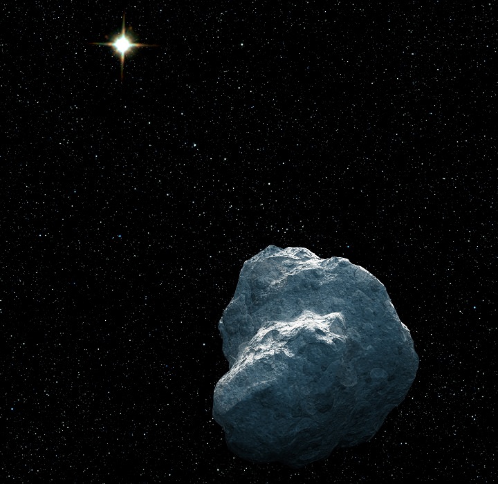
This is an artist’s concept of a craggy piece of solar system debris that belongs to a class of bodies called trans-Neptunian objects (TNOs). Credit: NASA
It will then expand more rapidly over about half a billion years until it is over two hundred times larger than it is today, and a couple of thousand times more luminous. This then starts the red-giant-branch (RGB) phase which will last around a billion years, during which time the the Sun will lose around a third of its mass.
During that time, many objects in the Kuiper Belt will warm up significantly, which will include Pluto, Eris, and countless other Trans-Neptunian Objects (TNOs).
However, given the composition of these bodies, and the relatively short window in which they will be warmer and wetter, it is not likely that life will evolve from scratch. Instead, we would probably have to transport it there from Earth, assuming humanity is still living, and seed Pluto and other surviving bodies with vegetation and terrestrial organisms.
In short, the best answer to the question – is there life on Pluto? – is a resounding maybe. Another possible answer is maybe not, with the caveat that there may indeed be life there someday (i.e. us, if we’re still around). In the meantime, all we can do is wait for data to begin coming in from New Horizons, and scan it for the telltale signs that life is indeed there right now!
New Horizons' last look at Pluto's Charon-facing hemisphere reveals the highest resolution view of four intriguing darks spots for decades to come. This image, taken early the morning of July 11, 2015, shows newly-resolved linear features above the equatorial region that intersect, suggestive of polygonal shapes. This image was captured when the spacecraft was 2.5 million miles (4 million kilometers) from Pluto. Credit: NASA/JHUAPL/SWRI
New Horizons’ last look at Pluto’s Charon-facing hemisphere reveals the highest resolution view of four intriguing darks spots for decades to come. This image, taken early the morning of July 11, 2015, shows newly-resolved linear features above the equatorial region that intersect, suggestive of polygonal shapes. This image was captured when the spacecraft was 2.5 million miles (4 million kilometers) from Pluto. Credit: NASA/JHUAPL/SWRI
Story updated[/caption]
The four puzzling spots (see above) are located on the hemisphere of Pluto which always faces its largest moon, Charon, and have captivated the scientists and public alike. Pluto and Charon are gravitationally locked with an orbital period of 6.4 days.
Over only the past few days, we are finally witnessing an amazing assortment of geological wonders emerge into focus from these never before seen worlds – as promised by the New Horizons team over a decade ago.
Be sure to take a good hard look at the image, because these spots and Pluto’s Charon-facing hemisphere will not be visible to New Horizons cameras and spectrometers during the historic July 14 encounter as the spacecraft whizzes by the binary worlds at speeds of some 30,800 miles per hour (more than 48,600 kilometers per hour) for their first up close reconnaissance.
And it’s likely to be many decades before the next visitor from Earth arrives at the frigid worlds at the far flung reaches of our solar system for a longer look, hopefully from orbit.
“The [July 11] image is the last, best look that anyone will have of Pluto’s far side for decades to come,” said New Horizons principal investigator Alan Stern of the Southwest Research Institute, Boulder, Colorado, in a statement.
The image of the mysterious spots was taken earlier today (July 11) by New Horizons Long Range Reconnaissance Imager (LORRI) at a distance of 2.5 million miles (4 million kilometers) from Pluto, and just released by NASA. The image resolution is 10 miles per pixel. One week ago it was only 40 miles per pixel.
They were first seen only in very recent LORRI images as Pluto’s disk finally was resolved and are located in a Missouri sized area about 300 miles (480 kilometers) across and above the equatorial region.
But until today they were still rather fuzzy – see image below from July 3! What a difference a few million miles (km) makes!
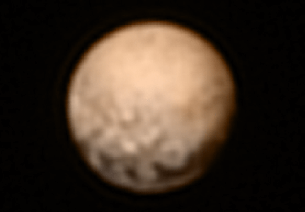
Latest color image of Pluto taken on July 3, 2015. Best yet image of Pluto was taken by the LORRI imager on NASA’s New Horizons spacecraft on July 3, 2015 at a distance of 7.8 million mi (12.5 million km), just prior to the July 4 anomaly that sent New Horizons into safe mode. Color data taken from the Ralph instrument gathered earlier in the mission. Credit: NASA/JHUAPL/SWRI
“The Pluto system is totally unknown territory,” said Dr. John Spencer, New Horizons co-investigator at today’s (July 11) daily live briefing from NASA and the New Horizons team.
“Pluto is like nowhere we’ve even been before. It is unlike anything we’ve visited before.”
Now, with the $700 million NASA planetary probe millions of miles closer to the double planet, the picture resolution has increased dramatically and the team can at least speculate.
Researchers say the quartet of “equally spaced” dark splotches are “suggestive of polygonal shapes” and the “boundaries between the dark and bright terrains are irregular and sharply defined.”
“It’s weird that they’re spaced so regularly,” says New Horizons program scientist Curt Niebur at NASA Headquarters in Washington.
However their nature remains “intriguing” and truly “unknown.”
“We can’t tell whether they’re plateaus or plains, or whether they’re brightness variations on a completely smooth surface,” added Jeff Moore of NASA’s Ames Research Center, Mountain View, California.
“It’s amazing what we are seeing now in the images, showing us things we’ve never seen before,” said Spencer.
“Every day we see things we never knew before. We see these crazy black and white patterns. And we have no idea what these mean.”
Answering these questions and more is what the encounter is all about.
Pluto is just chock full of mysteries, with new ones emerging every day as New Horizons at last homes in on its quarry, and the planet grows from a spot to an enlarging disk with never before seen surface features, three billion miles from Earth after an interplanetary journey of some nine and a half years.
“We see circular things and wonder are those craters? Or are they something else,” Spencer elaborated.
“We saw circular features on Neptune’s moon Triton that are not craters. So we should know in a few days . But right now we are just having an awful lot of fun just speculating. It’s just amazing.”
Until a few days ago, we didn’t know that “the other Red Planet” had a big bright heart and a dark ‘whale-shaped’ feature – see my earlier articles; here and here.
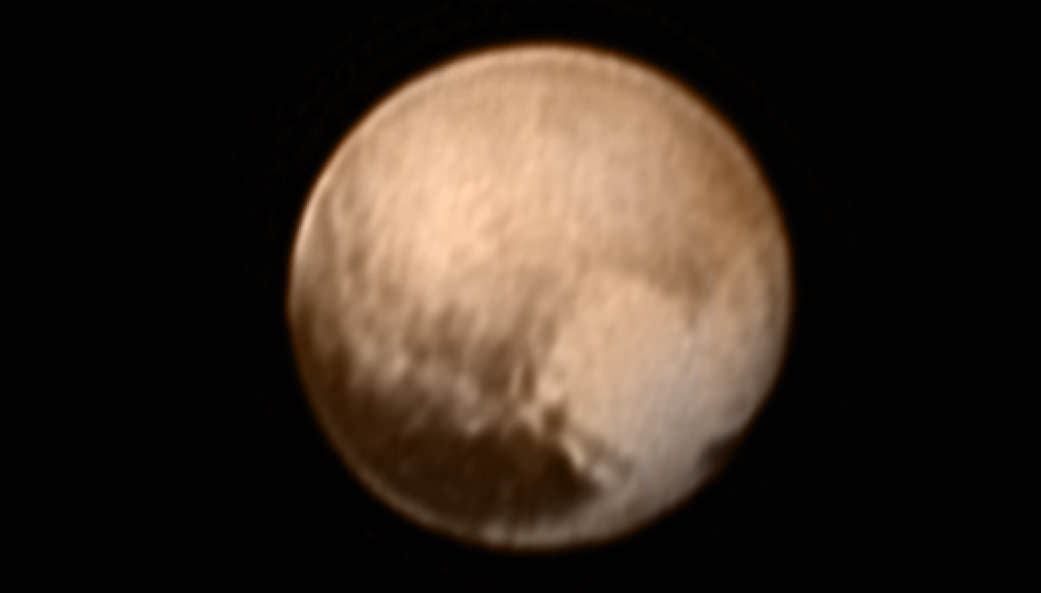
Pluto’s “Heart” is seen in this new image from New Horizons’ Long Range Reconnaissance Imager (LORRI) received on July 8, 2015 after normal science operations resumed following the scary July 4 safe mode anomaly that briefing shut down all science operations. The LORRI image has been combined with lower-resolution color information from the Ralph instrument. Credits: NASA-JHUAPL-SWRI
“When we combine images like this of the far side with composition and color data the spacecraft has already acquired but not yet sent to Earth, we expect to be able to read the history of this face of Pluto,” Moore explained.
New Horizons will swoop to within about 12,500 kilometers (nearly 7,750 miles) of Pluto’s surface and about 17,900 miles (28,800 kilometers) from Charon during closest approach at approximately 7:49 a.m. EDT (11:49 UTC) on July 14.
The probe was launched back on Jan. 19, 2006 on a United Launch Alliance Atlas V rocket on a 9 year voyage of over 3.6 billion miles (5.7 billion km).
Pluto is the last of the nine classical planets to be explored up close and completes the initial the initial reconnaissance of the solar system nearly six decades after the dawn of the space age. It represents a whole new class of objects.
“Pluto is a member of a whole new family of objects,” said Jim Green, director of Planetary Science, NASA Headquarters, Washington, in today’s live Pluto update.
“We call that the Kuiper Belt. And it is the outer solar system.”
New Horizons is equipped with a suite of seven science instruments gathering data during the approach and encounter phases with the Pluto system.
Graphic shows data gathered by New Horizons particle and plasma science instruments from 2 million miles out on July 11, 2015. Credit: NASA/JHUAPL/SWRI
The New Frontiers spacecraft was built by a team led by Stern and included researchers from SwRI and the Johns Hopkins University Applied Physics Laboratory (APL) in Laurel, Maryland. APL also operates the New Horizons spacecraft and manages the mission.
Stay tuned here for Ken’s continuing Earth and planetary science and human spaceflight news.
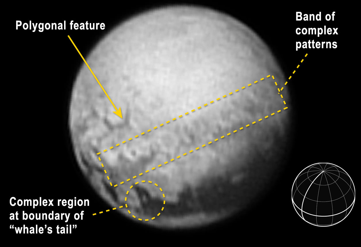
Tantalizing signs of geology on Pluto are revealed in this image from New Horizons taken on July 9, 2015 from 3.3 million miles (5.4 million km) away. This annotated version shows the large dark feature nicknamed “the whale” that straddles Pluto’s equator, a swirly band and a curious polygonal outline. At lower is a reference globe showing Pluto’s orientation in the image, with the equator and central meridian in bold. Credit: NASA-JHUAPL-SWRI
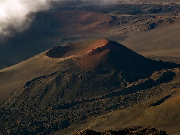
Haleakala, a giant shield volcano, forms the eastern bulwark of the island of Maui. Any volcanoes on an asteroid would not form large cones like this. Credit: National Geographic/Cathy Roberts
Hawaii is famous for its lovely mountains, tropical climate, and majestic oceanfront vistas. Another thing it is famous for is the string of volcanoes that dot its islands. As a land that sits atop a geographic hot spot – i.e. an area deep within the Earth’s mantle from which heat rises, forming magma that is then pushed to the surface – the island is also home to some serious volcanic activity.
Consider Haleakala, the massive shield volcano that constitutes more than 75% of the Hawaiian Island of Maui. The result of volcanic activity that took place roughly 1 million years ago, this volcano has played an active role in the geological and cultural history of the Hawaiian islands. Description and Naming: Like all shield volcanoes, Haleakala was formed from a series of highly fluid magma flows. This is the reason for its general appearance, as well as the designation – i.e. it resembles a broad shield lying on the ground. It’s tallest peak, which is named is Pu’u ‘Ula’ula (“Red Hill”) in native Hawaiian, measures 3,055 m (10,023 ft) tall.
At Haleakala’s summit lies a massive depression (crater) that measures some 11.25 km (7 miles) in diameter and nearly 800 m (2,600 ft) deep. The name Haleakala means literally “House of the Sun”, which was given to the general mountain area by the early Hawaiian people.
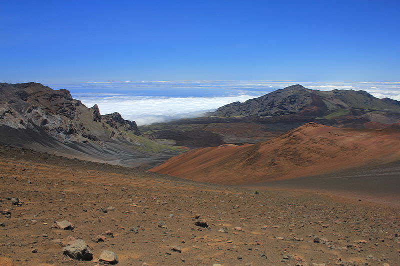
Sliding sands trail in the Haleakala Crater, Maui. Credit: Haleakala National Park
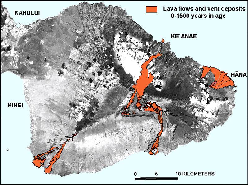
Geology: Haleakala is part of a sequence of lava flows that emerged near the end of East Maui. This region is believed to have begun experiencing lava flows about 2.0 million years ago, and it is estimated that the volcano formed from the ocean floor to its current shield-like shape over the course of the ensuing 600,000 years. The oldest exposed lava flow on East Maui is dated to 1.1 million years ago.
In the past 30,000 years, the volcanism on East Maui has been focused along the southwest and east rift zones. These two volcanic axes together form one gently curving arc that passes from La Perouse Bay (southwest flank of East Maui) through Haleakala Crater to Hana on the east flank.
The alignment of these axes continues east beneath the ocean as Haleakala Ridge, one of the longest rift zones along the Hawaiian Islands volcanic chain. The on-land segment of this lengthy volcanic line of vents is the zone of greatest hazard for future lava flows and cindery ash.
Contrary to popular belief, the Haleakala “crater” is not volcanic in origin, nor can it accurately be called a caldera (which is formed when the summit of a volcano collapses to form a depression). Scientists believe instead that the depression was formed when the headwalls of two large erosional valleys merged at the summit of the volcano.
Modern techniques have allowed geologists to accurately date the lava flows on Maui. Credit: D. Sherrod/USGS
History: Haleakala has produced numerous eruptions in the last 30,000 years, including in the last 500 years. The volcano has figured prominently in the island’s history of human occupation. In Hawaiian folklore, the crater at the summit was home to the grandmother of the demigod Maui. According to the legend, Maui’s grandmother helped him capture the sun and force it to slow its journey across the sky in order to lengthen the day.
Until recently, the East Maui Volcano was thought to have last erupted around 1790, based largely on comparisons of maps made during the voyages of the explorers La Perouse and George Vancouver. Recent advanced dating tests, however, have shown that the last eruption was more likely to have taken place in the 17th century.
Modern geologic mapping efforts began in 1997, which yielded the most detailed and accurate picture of Haleakala’s volcanic history to date. In addition, there are fears that the volcano is not extinct, but just currently dormant, and may erupt again within the next 500 years.
For these reasons, the U.S. Geological Survey maintains a sparse seismic network on Haleakala volcano and conducts periodic surveys, using GPS receivers that gather data about the volcano’s surface deformation or lack thereof.
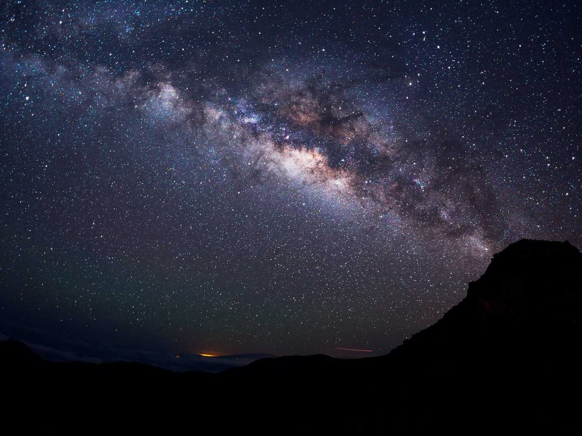
The view from Haleakala at night, Haleakala National Park. Credit: travelbloggerbuzz.com
Modern Uses: In 1916, Haleakala National Park was created, a 30,183-acre (122.15 km2) park surrounding the summit depression, Kipahulu Valley on the southeast, and ‘Ohe‘o Gulch (and pools), extending to the shoreline in the Kipahulu area. Within the park, 19,270 acres (77.98 km2) is a wilderness area, which is why the park area was designated an International Biosphere Reserve in 1980.
The main feature of this part of the park is the famous Haleakala Crater. Two main trails lead into the crater from the summit area – the Halemau’u and Sliding Sands trails. Haleakala is popular with tourists and locals alike, who often venture to its summit – or to the visitor center just below the summit – to view the sunrise. There is lodging in the crater in the form of a few simple cabins.
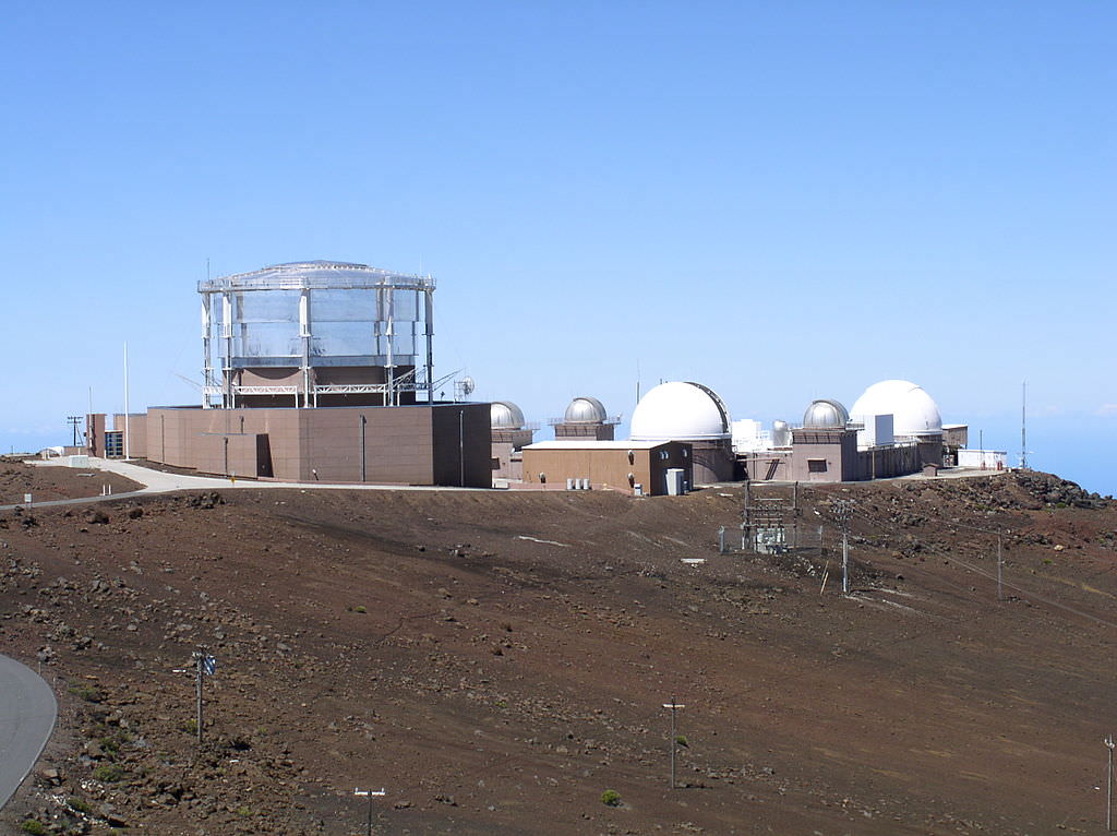
Because of the clarity and stillness of the air, the summit of Haleakala is one of the most valuable spots for observatories. It is also far enough away from the city lights to avoid light pollution, and above one-third of the planet’s atmosphere. Hence why the summit is the location of an astrophysical research facility – known as “Science City” – which is operated by a number of U.S. government and academic organizations.
These include the U.S. Department of Defense, the University of Hawaii, the Smithsonian Institution, the US Air Force, the Federal Aviation Administration (FAA), and others. Some of the telescopes operated by the US Department of Defense are involved in researching man-made (e.g. spacecraft, monitoring satellites, rockets, and laser technology) rather than celestial objects.
The Science City research faciltiy, located at the summit of the Haleakala volcano. Credit: Wikipedia Commons/Tawker
The scientific program is run in collaboration with defense contractors in the Maui Research and Technology Park in Kihei. Despite concerns that Maui’s growing population will mean increased incidents of light pollution, new telescopes are being added – such as the Pan-STARRS in 2006.
Although another 500 years or more may pass before Haleakala erupts again, it’s also possible that new eruptions will begin in the near future. However, according to the United States Geological Survey (USGS) Volcano Warning Scheme for the United States, the Volcanic-Alert Level as of June 2013 was “normal”. Given the likelihood of significant environmental and property damage, not to mention the potential loss of life, one can only hope this holds true for the foreseeable future.
Tantalizing signs of geology on Pluto are revealed in this image from New Horizons taken on July 9, 2015 from 3.3 million miles (5.4 million km) away. This annotated version shows the large dark feature nicknamed "the whale" that straddles Pluto's equator, a swirly band and a curious polygonal outline. At lower is a reference globe showing Pluto’s orientation in the image, with the equator and central meridian in bold. Credit: NASA-JHUAPL-SWRI
Bit by the Pluto bug? Day by day, new images appear showing an ever clearer view of a world we inexplicably love. Call it a dwarf planet. Call it a planet. It’s the unknown, and we can’t help but be drawn there.
Pluto made history when it was discovered in 1930. In 2015, it’s doing it all over again. Check out the new geology peeping into view.I’m reminded of the early explorers who shoved off in wooden ships in search of land across the water. After a long and often perilous journey, the mists would finally clear and the dark outline of land take form in the distance. It’s been 9 1/2 years since our collective Pluto voyage began. Yeah, we’re almost there.
Science team members react to the latest image of Pluto at the Johns Hopkins University Applied Physics Lab on July 10, 2015. Left to right: Cathy Olkin, Jason Cook, Alan Stern, Will Grundy, Casey Lisse, and Carly Howett. Credit: Michael Soluri
Today’s image release clearly shows a world growing more geologically diverse by the day.
“We’re close enough now that we’re just starting to see Pluto’s geology,” said New Horizons program scientist Curt Niebur, on NASA’s website. Niebur, who’s keenly interested in the gray area just above the whale’s “tail” feature, called it a “unique transition region with a lot of dynamic processes interacting, which makes it of particular scientific interest.”
The non-annotated version of the top photo. The ‘whale’ lies near the dwarf planet’s equator. Pluto’s axis is tilted 123° to its orbital plane. Credit: NASA-JHUAPL-SWRI
Not only that, but the new photo shows an approximately 1,000-mile-long band of swirly terrain crossing the planet from east to northeast, a large, polygonal (roughly hexagonal) feature and new textures within the ‘whale’.
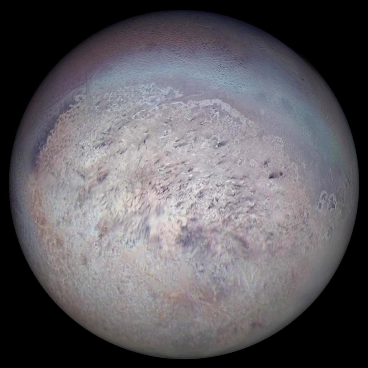
Neptune’s largest moon Triton photographed on August 25, 1989 by Voyager 2. Triton has a surface of mostly frozen nitrogen, a water ice-rich crust, an icy mantle and rock-metal core. Credit: NASA
Even to a layperson’s eye, Pluto’s terrain appears very different from that of Ceres or Vesta. In trying to make sense of what we see, Neptune’s moon Triton may be our best Plutonian analog with its frosts, weird cantaloupe terrain and an assortment of dark patches, some produced by icy volcanism.
New Horizons was about 3.7 million miles (6 million kilometers) from Pluto and Charon when it snapped this portrait late on July 8, 2015. Credits: NASA-JHUAPL-SWRI
Other recent photos include this pretty view of Charon and Triton snapped late on July 8. NASA describes them eloquently as “two icy worlds, spinning around their common center of gravity like a pair of figure skaters clasping hands.” Charon and all of Pluto’s known moons formed from debris released when another planet struck Pluto long ago. New Horizons principal investigator Alan Stern attributes its bland color to its composition — mostly water ice. Pluto in contrast has a mantle of water ice, but it’s coated with methane, nitrogen and carbon dioxide ices and possibly organic compounds, too.
Color photos of Pluto and Charon side by side. The arcs along Pluto’s right limb are artifacts but not the white border along the bottom. Could it be frost? Credit: NASA-JHUAPL-SWRI
Sarychev volcano, (located in Russia's Kuril Islands, northeast of Japan) in an early stage of eruption on June 12, 2009. Credit: NASA
What if someone were to tell you that there’s a region in the world where roughly 90% of the world’s earthquakes occur. What if they were to tell you that this region is also home to over 75% of the world’s active and dormant volcanoes, and all but 3 of the world’s 25 largest eruptions in the last 11,700 years took place here.
Chances are, you’d think twice about buying real-estate there. But strangely enough, hundreds of millions of people live in this area, and some of the most densely-packed cities in the world have been built atop its shaky faults. We are talking about the Pacific Ring of Fire, a geologically and volcanically active region that stretches from one side of the Pacific to the other.
Definition:
Also known as the circum-Pacific belt, the “Ring of Fire” is a 40,000 km (25,000 mile) horseshoe-shaped basin that is associated with a nearly continuous series of oceanic trenches, volcanic arcs, and volcanic belts and/or plate movements. This ring accounts for 452 volcanoes (active and dormant), stretching from the southern tip of South America, up along the coast of North America, across the Bering Strait, down through Japan, and into New Zealand – with several active and dormant volcanoes in Antarctica closing the ring.
Tectonic Activity:
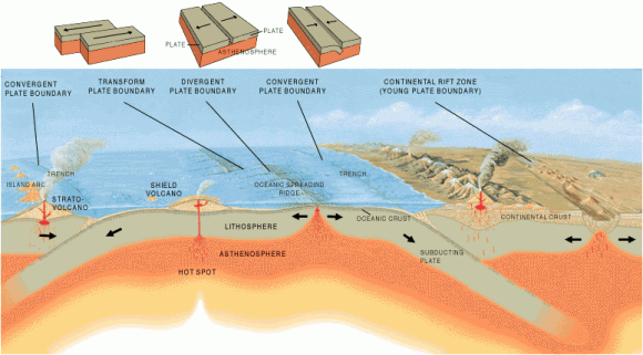
The Ring of Fire is the direct result of plate tectonics and the movement and collisions of lithospheric plates. These plates, which constitute the outer layer of the planet, are constantly in motion atop the mantle. Sometimes they collide, pull apart, or slide alongside each other; resulting in convergent boundaries, divergent boundaries, and transform boundaries.
The Pacific Ring of Fire, a string of volcanic regions extending from the South Pacific to South America. Credit: Public Domain
In the case of the former, subduction zones are often the result, where the heavier plate slips under the lighter plate – forming a deep trench. This subduction changes the dense mantle into buoyant magma, which rises through the crust to the Earth’s surface. Over millions of years, this rising magma creates a series of active volcanoes known as a volcanic arc.
These ocean trenches and volcanic arcs run parallel to one another. For instance, the Aleutian Islands in the U.S. state of Alaska run parallel to the Aleutian Trench. Both geographic features continue to form as the Pacific Plate subducts beneath the North American Plate. Meanwhile, the Andes Mountains of South America run parallel to the Peru-Chile Trench, created as the Nazca Plate subducts beneath the South American Plate.
In the case of divergent boundaries, these are formed when tectonic plates pull apart, forming rift valleys on the seafloor. When this happens, magma wells up in the rift as the old crust pulls itself in opposite directions, where it is cooled by seawater to form new crust. This upward movement and eventual cooling of this magma has created high ridges on the ocean floor over millions of years.
The East Pacific Rise is a site of major seafloor spreading in the Ring of Fire, located on the divergent boundary of the Pacific Plate and the Cocos Plate (west of Central America), the Nazca Plate (west of South America), and the Antarctic Plate. The largest known group of volcanoes on Earth is found underwater along the portion of the East Pacific Rise between the coasts of northern Chile and southern Peru.
The different type of tectonic plate boundaries. Credit: oceanexplorer.noaa.gov
A transform boundary is formed when tectonic plates slide horizontally and parts get stuck at points of contact. Stress builds in these areas as the rest of the plates continue to move, which causes the rock to break or slip, suddenly lurching the plates forward and causing earthquakes. These areas of breakage or slippage are called faults, and the majority of Earth’s faults can be found along transform boundaries in the Ring of Fire.
The San Andreas Fault, stretching along the central west coast of North America, is one of the most active faults on the Ring of Fire. It lies on the transform boundary between the North American Plate, which is moving south, and the Pacific Plate, which is moving north. Measuring about 1,287 kilometers (800 miles) long and 16 kilometers (10 miles) deep, the fault cuts through the western part of the U.S. state of California.
Plate Boundaries:
The eastern section of the Ring of Fire is the result of the Nazca Plate and the Cocos Plate being subducted beneath the westward moving South American Plate. Meanwhile, the Cocos Plate is being subducted beneath the Caribbean Plate, in Central America. A portion of the Pacific Plate along with the small Juan de Fuca Plate are being subducted beneath the North American Plate.
Along the northern portion, the northwestward-moving Pacific plate is being subducted beneath the Aleutian Islands arc. Farther west, the Pacific plate is being subducted along the Kamchatka Peninsula arcs on south past Japan.
The Earth’s Tectonic Plates. Credit: msnucleus.org
The southern portion is more complex, with a number of smaller tectonic plates in collision with the Pacific plate from the Mariana Islands, the Philippines, Bougainville, Tonga, and New Zealand. This portion excludes Australia, since it lies in the center of its tectonic plate.
Indonesia lies between the Ring of Fire along the northeastern islands adjacent to and including New Guinea and the Alpide belt along the south and west from Sumatra, Java, Bali, Flores, and Timor. The famous and very active San Andreas Fault zone of California is a transform fault which offsets a portion of the East Pacific Rise under southwestern United States and Mexico.
Volcanic Activity:
Most of the active volcanoes on The Ring of Fire are found on its western edge, from the Kamchatka Peninsula in Russia, through the islands of Japan and Southeast Asia, to New Zealand. Mount Ruapehu in New Zealand is one of the more active volcanoes in the Ring of Fire, with yearly minor eruptions, and major eruptions occurring about every 50 years.
Krakatau, perhaps better known as Krakatoa, is an island volcano in Indonesia. Krakatoa erupts less often than Mount Ruapehu, but much more spectacularly. Beneath Krakatoa, the denser Australian Plate is being subducted beneath the Eurasian Plate. An infamous eruption in 1883 destroyed the entire island, sending volcanic gas, volcanic ash, and rocks as high as 80 kilometers (50 miles) in the air. A new island volcano, Anak Krakatau, has been forming with minor eruptions ever since.
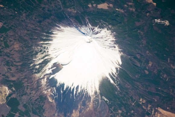
Mount Fuji, Japan, as seen from the ISS. Credit: NASA
Mount Fuji, Japan’s tallest and most famous mountain, is an active volcano in the Ring of Fire. Mount Fuji last erupted in 1707, but recent earthquake activity in eastern Japan may have put the volcano in a “critical state.” Mount Fuji sits at a “triple junction,” where three tectonic plates (the Amur Plate, Okhotsk Plate, and Philippine Plate) interact.
The Ring of Fire’s eastern half also has a number of active volcanic areas, including the Aleutian Islands, the Cascade Mountains in the western U.S., the Trans-Mexican Volcanic Belt, and the Andes Mountains. Mount St. Helens, in the U.S. state of Washington, is an active volcano in the Cascade Mountains.
Below Mount St. Helens, both the Juan de Fuca and Pacific plates are being subducted beneath the North American Plate. Its historic 1980 eruption lasted 9 hours and covered 11 U.S. states with tons of volcanic ash. The eruption caused the deaths of 57 people, over a billion dollars in property damage, and reduced hundreds of square miles to wasteland.
Popocatépetl is one of the most active and dangerous volcanoes in the Ring of Fire, with 15 recorded eruptions since 1519. The volcano lies on the Trans-Mexican Volcanic Belt, which is the result of the small Cocos Plate subducting beneath the North American Plate. Located close to the urban areas of Mexico City and Puebla, Popocatépetl poses a risk to the more than 20 million people that live close enough to be threatened by a destructive eruption.
Map of the Earth showing the relation between fault lines (blue) and zones of volcanic activity (red). Credit: zmescience.com
Earthquakes:
Scientists have known for some time that the majority of the seismic activity occurs along plate boundaries. Hence why roughly 90% of the world’s earthquakes – which is estimated to be around 500,000 a year, one-fifth of which are detectable – occur around the Pacific Rim, where multiple plate boundaries exist.
As a result, earthquakes are a regular occurrence in places like Japan, Indonesia and New Zealand in Asia and the South Pacific; Alaska, British Columbia, California and Mexico in North America; and El Salvador, Guatemala, Peru and Chile in Central and South America. Where fault lines run beneath the ocean, larger earthquakes in these regions also trigger tsunamis.
The most well-known tsumanis to take place in the Ring of Fire include the 2004 Indian Ocean earthquake and tsunami. This was the most devastating tsunami of its kind in modern times, killing around 230,000 people and laying waste to communities throughout Indonesia, Thailand, and Southern Asia.
In 2010, an earthquake triggered a tsunami which caused 4334 confirmed deaths and devastating several coastal towns in south-central Chile, including the port at Talcahuano. The earthquake also generated a blackout that affected 93 percent of the Chilean population.
In 2011, an earthquake off the Pacific coast of Tohoku led to a tsunami that struck Japan and led to 5,891 deaths, 6,152 injuries, and 2,584 people to be declared missing across twenty prefectures. The tsunami also caused meltdowns at three reactors in the Fukushima Daiichi Nuclear Power Plant complex.
The Ring of Fire is a crucial region for many reasons. It serves as one of the main boundary regions for the tectonic plates of over half of the globe. It also affects the lives of millions if not billions of people who live in these regions. For many of the people who live in the Pacific Ring of Fire, the reality of a volcanic eruption or earthquake is commonplace and a challenge they have come to deal with over time.
At the same time, the volcanic activity has also provided many valuable resources, such as rich farmland and the possibility of tapping geothermal activity for heating and electricity. As always, nature gives with one hand and takes with the other!
If you have enjoyed this article there are several others on Universe Today that you will find interesting. Here is one called 10 Interesting Facts About Volcanoes. There is also a great article about plate tectonics.
You can also find some good resources online. There is a companion site for the PBS program Savage Earth that talks about the Ring of Fire. You can also check out the USGS site to see a detailed map of the Pacific Ring of Fire and more detailed information about plate tectonics.
You can also listen to Astronomy Cast. Episode 141 talks about volcanoes.