Astronomy Archives

December 15, 2014December 23, 2015 by Vanessa Janek

New Signal May Be Evidence of Dark Matter, Say Researchers

Dark Matter Halo and dwarf galaxies — All galaxies are thought to have a dark matter halo. This image shows the distribution of dark matter surrounding our very own Milky Way. Image credit: J. Diemand, M. Kuhlen and P. Madau (UCSC)

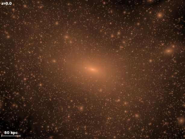
Dark matter is the architect of large-scale cosmic structure and the engine behind proper rotation of galaxies. It’s an indispensable part of the physics of our Universe – and yet scientists still don’t know what it’s made of. The latest data from Planck suggest that the mysterious substance comprises 26.2% of the cosmos, making it nearly five and a half times more prevalent than normal, everyday matter. Now, four European researchers have hinted that they may have a discovery on their hands: a signal in x-ray light that has no known cause, and may be evidence of a long sought-after interaction between particles – namely, the annihilation of dark matter.

When astronomers want to study an object in the night sky, such as a star or galaxy, they begin by analyzing its light across all wavelengths. This allows them to visualize narrow dark lines in the object’s spectrum, called absorption lines. Absorption lines occur because a star’s or galaxy’s component elements soak up light at certain wavelengths, preventing most photons with those energies from reaching Earth. Similarly, interacting particles can also leave emission lines in a star’s or galaxy’s spectrum, bright lines that are created when excess photons are emitted via subatomic processes such as excitement and decay. By looking closely at these emission lines, scientists can usually paint a robust picture of the physics going on elsewhere in the cosmos.

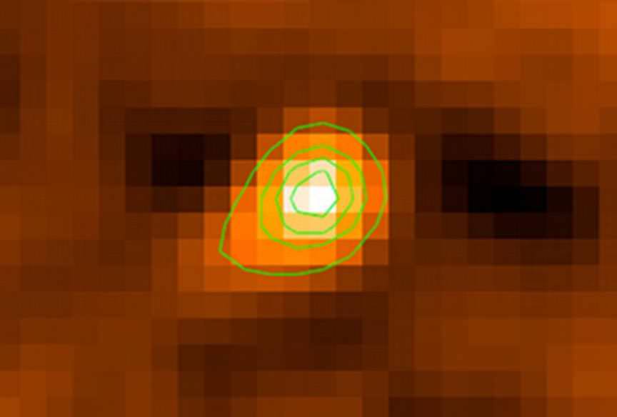
But sometimes, scientists find an emission line that is more puzzling. Earlier this year, researchers at the Laboratory of Particle Physics and Cosmology (LPPC) in Switzerland and Leiden University in the Netherlands identified an excess bump of energy in x-ray light coming from both the Andromeda galaxy and the Perseus star cluster: an emission line with an energy around 3.5keV. No known process can account for this line; however, it is consistent with models of the theoretical sterile neutrino – a particle that many scientists believe is a prime candidate for dark matter.

The researchers believe that this strange emission line could result from the annihilation, or decay, of these dark matter particles, a process that is thought to release x-ray photons. In fact, the signal appeared to be strongest in the most dense regions of Andromeda and Perseus and increasingly more diffuse away from the center, a distribution that is also characteristic of dark matter. Additionally, the signal was absent from the team’s observations of deep, empty space, implying that it is real and not just instrumental artifact.

In a pre-print of their paper, the researchers are careful to stress that the signal itself is weak by scientific standards. That is, they can only be 99.994% sure that it is a true result and not just a rogue statistical fluctuation, a level of confidence that is known as 4σ. (The gold standard for a discovery in science is 5σ: a result that can be declared “true” with 99.9999% confidence) Other scientists are not so sure that dark matter is such a good explanation after all. According to predictions made based on measurements of the Lyman-alpha forest – that is, the spectral pattern of hydrogen absorption and photon emission within very distant, very old gas clouds – any particle purporting to be dark matter should have an energy above 10keV – more than twice the energy of this most recent signal.

As always, the study of cosmology is fraught with mysteries. Whether this particular emission line turns out to be evidence of a sterile neutrino (and thus of dark matter) or not, it does appear to be a signal of some physical process that scientists do not yet understand. If future observations can increase the certainty of this discovery to the 5σ level, astrophysicists will have yet another phenomena to account for – an exciting prospect, regardless of the final result.

The team’s research has been accepted to Physical Review Letters and will be published in an upcoming issue.

December 15, 2014December 23, 2015 by Matt Williams

Just in Time for the Holidays – Galactic Encounter Puts on Stunning Display

That's the case with NGC 2207 and IC 2163, which are located about 130 million light-years from Earth, in the constellation of Canis Major. Image credit: NASA/CXC/SAO/STScI/JPL-Caltech

At this time of year, festive displays of light are to be expected. This tradition has clearly not been lost on the galaxies NHC 2207 and IC 2163. Just in time for the holidays, these colliding galaxies, which are located within the Canis Major constellation (some 130 million light-years from Earth,) were seen putting on a spectacular lights display for us folks here on Earth!

And while this galaxy has been known to produce a lot of intense light over the years, the image above is especially luminous. A composite using data from the Chandra Observatory and the Hubble and Spitzer Space Telescopes, it shows the combination of visible, x-ray, and infrared light coming from the galactic pair.

In the past fifteen years, NGC 2207 and IC 2163 have hosted three supernova explosions and produced one of the largest collections of super bright X-ray lights in the known universe. These special objects – known as “ultraluminous X-ray sources” (ULXs) – have been found using data from NASA’s Chandra X-ray Observatory.

While the true nature of ULXs is still being debated, it is believed that they are a peculiar type of star X-ray binary. These consist of a star in a tight orbit around either a neutron star or a black hole. The strong gravity of the neutron star or black hole pulls matter from the companion star, and as this matter falls toward the neutron star or black hole, it is heated to millions of degrees and generates X-rays.

the core of galaxy Messier 82 (M82), where two ultraluminous X-ray sources, or ULXs, reside (X-1 and X-2). Credit: NASA — *The core of galaxy Messier 82 (M82), where two ultraluminous X-ray sources, or ULXs, reside (X-1 and X-2). Credit: NASA*

Data obtained from Chandra has determined that – much like the Milky Way Galaxy – NGC 2207 and IC 2163 are sprinkled with many star X-ray binaries. In the new Chandra image, this x-ray data is shown in pink, which shows the sheer prevalence of x-ray sources within both galaxies.

Meanwhile, optical light data from the Hubble Space Telescope is rendered in red, green, and blue (also appearing as blue, white, orange, and brown due to color combinations,) and infrared data from the Spitzer Space Telescope is shown in red.

The Chandra observatory spent far more time observing these galaxies than any previous ULX study, roughly five times as much. As a result, the study team – which consisted of researchers from Harvard University, MIT, and Sam Houston State University – were able to confirm the existence of 28 ULXs between NGC 2207 and IC 2163, seven of which had never before been seen.

In addition, the Chandra data allowed the team of scientists to observe the correlation between X-ray sources in different regions of the galaxy and the rate at which stars are forming in those same regions.

Galaxy mergers, such as the Mice Galaxies will be part of Galaxy Zoo's newest project. Credit: Hubble Space Telescope — *The Mice galaxies, seen here well into the process of merging. Credit: Hubble Space Telescope*

As the new Chandra image shows, the spiral arms of the galaxies – where large amounts of star formation is known to be occurring – show the heaviest concentrations of ULXs, optical light, and infrared. This correlation also suggests that the companion star in the star X-ray binaries is young and massive.

This in turn presents another possibility which has to do with star formation during galactic mergers. When galaxies come together, they produce shock waves that cause clouds of gas within them to collapse, leading to periods of intense star formation and the creation of star clusters.

The fact that the ULXs and the companion stars are young (the researchers estimate that they are only 10 million years old) would seem to confirm that they are the result of NGC 2207 and IC 2163 coming together. This seem a likely explanation since the merger between these two galaxies is still in its infancy, which is attested to by the fact that the galaxies are still separate.

They are expected to collide soon, a process which will make them look more like the Mice Galaxies (pictured above). In about one billion years time, they are expected to finish the process, forming a spiral galaxy that would no doubt resemble our own.

A paper describing the study was recently published on online with The Astrophysical Journal.

Further Reading: NASA/JPL, Chandra, arXiv Astrophysics

December 11, 2014December 23, 2015 by Tim Reyes

Rosetta’s Instruments Direct Scientists to Look Elsewhere for the Source of Earth’s Water

Illustration of a rocky planet being bombarded by comets. (Image credit: NASA/JPL-Caltech)

Where did all of our water come from? What might seem like a simple question has challenged and intrigued planetary scientists for decades. So results just released by Rosetta mission scientists have been much anticipated and the observations of the Rosetta spacecraft instruments are telling us to look elsewhere. The water of comet 67P/Churyumov-Gerasimenko does not resemble Earth’s water.

Because the Earth was extremely hot early in its formation, scientists believe that Earth’s original water should have boiled away like that from a boiling kettle. Prevailing theories have considered two sources for a later delivery of water to the surface of the Earth once conditions had cooled. One is comets and the other is asteroids. Surely some water arrived from both sources, but the question has been which one is the predominant source.

There are two areas of our Solar System in which comets formed about 4.6 billion years ago. One is the Oort cloud far beyond Pluto. Everything points to Comet 67P’s origins being the other birthplace of comets – the Kuiper Belt in the region of Neptune and Pluto. The Rosetta results are ruling out Kuiper Belt comets as a source of Earth’s water. Previous observations of Oort cloud comets, such as Hyakutake and Hale-Bopp, have shown that they also do not have Earth-like water. So planetary scientists must reconsider their models with weight being given to the other possible source – asteroids.

The question of the source of Earth’s water has been tackled by Earth-based instruments and several probes which rendezvous with comets. In 1986, the first flyby of a comet – Comet 1P/Halley, an Oort cloud comet – revealed that its water was not like the water on Earth. How the water from these comets –Halley’s and now 67P – differs from Earth’s is in the ratio of the two types of hydrogen atoms that make up the water molecule.

Illustration of the Rosetta spacecraft showing the location of the ROSINA mass spectrometer instrument, DFMS. The difference between a Deuterium and Hydrogen atom are also illustrated. A water molecule with Deuterium is known as heavy water due to the additional mass of D vs. H (an extra neutron). (Credit: ESA/Rosetta) — Illustration of the Rosetta spacecraft showing the location of the ROSINA mass spectrometer instrument, DFMS. The difference between a Deuterium and Hydrogen atom is also illustrated. A water molecule with Deuterium is known as heavy water due to the additional mass of Dueterium vs. Hydrogen (i.e., an extra neutron). (Credit: ESA/Rosetta)

Measurements by spectrometers revealed how much Deuterium – a heavier form of the Hydrogen atom – existed in relation to the most common type of Hydrogen in these comets. This ratio, designated as D/H, is about 1 in 6000 in Earth’s ocean water. For the vast majority of comets, remote or in-situ measurements have found a ratio that is higher which does not support the assertion that comets delivered water to the early Earth surface, at least not much of it.

Most recently, Hershel space telescope observations of comet Hartley 2 (103P/Hartley) caused a stir in the debate of the source of Earth’s water. The spectral measurements of the comet’s light revealed a D/H ratio just like Earth’s water. But now the Hershel observation has become more of an exception because of Rosetta’s latest measurements.

A plot displaying the Deuterium/Hydrogen (D/H) ratio of Solar System objects. Only asteroids have a D/H ratio that matches the Earths and comets with the exception of two so far measured have higher ratios. Objects are grouped by color. Planets & moons (blue), chrondritic meteorites from the asteroid belt (grey), Oort cloud comets(purple), Jupiter family comets(pink). Diamond markers = In Situ measurements, Circles = remote astronomical measurements(Credit: Altwegg et al. 2014) — A plot displaying the Deuterium/Hydrogen (D/H) ratio of Solar System objects. Asteroids have a D/H ratio that matches that of the Earth, while comets – except for two measured to date – have higher ratios. Objects are grouped by color: planets & moons (blue), chrondritic meteorites from the asteroid belt (grey), Oort cloud comets (purple), and Jupiter family comets (pink). Diamond markers = In Situ measurements; circles = remote astronomical measurements. (Credit: Altwegg, et al. 2014)

The new measurements of 67P were made by the ROSINA Double Focusing Mass Spectrometer (DFMS) on board Rosetta. Unlike remote observations using light which are less accurate, Rosetta was able to accurately measure the quantities of Deuterium and common Hydrogen surrounding the comet. Scientists could then simply determine a ratio. The results are reported in the paper “67P/Churyumov-Gerasimenko, a Jupiter Family Comet with a high D/H ratio” by K. Altwegg, et al., published in the 10 December 2014 issue of Science.

New Rosetta mission findings do not exclude comets as a source of water in and on the Earth's crust but does indicate comets were a minor contribution. A four-image mosaic comprises images taken by Rosetta’s navigation camera on 7 December from a distance of 19.7 km from the centre of Comet 67P/Churyumov-Gerasimenko. (Credit: ESA/Rosetta/Navcam Imager) — New Rosetta mission findings do not exclude comets as a source of water in and on the Earth’s crust but does indicate comets were a minor contribution. A four-image mosaic comprises images taken by Rosetta’s navigation camera on 7 December from a distance of 19.7 km from the centre of Comet 67P/Churyumov-Gerasimenko. (Credit: ESA/Rosetta/Navcam Imager)

The ROSINA instrument observations determined a ratio of 5.3 ± 0.7 × 10^-4, which is approximately 3 times the ratio of D/H for Earth’s water. These results do not exclude comets as a source of terrestrial water but they do redirect scientists to consider asteroids as the predominant source. While asteroids have much lower water content compared with comets, asteroids, and their smaller versions, meteoroids, are more numerous than comets. Every meteor/falling star that we see burning up in our atmosphere delivers a myriad of compounds, including water, to Earth. Early on, the onslaught of meteoroids and asteroids impacting Earth was far greater. Consequently, the small quantities of water added delivered by each could add up to what now lies in the oceans, lakes, streams, and even our bodies.

References:

D/H Ratio of Water on Earth Measured with DFMS

67P/Churyumov-Gerasimenko, a Jupiter family comet with a high D/H ratio

Rosetta fuels the debate on the Origin of Earth’s Water

The Provenances of Asteroids, and Their Contributions to the Volatile Inventories of the Terrestrial Planets

Recent Universe Today related article:

What Percent of Earth is Water?

December 11, 2014December 23, 2015 by Vanessa Janek

Gamma Ray Bursts Limit The Habitability of Certain Galaxies, Says Study

An artistic image of the explosion of a star leading to a gamma-ray burst. (Source: FUW/Tentaris/Maciej Fro?ow)

Gamma ray bursts (GRBs) are some of the brightest, most dramatic events in the Universe. These cosmic tempests are characterized by a spectacular explosion of photons with energies 1,000,000 times greater than the most energetic light our eyes can detect. Due to their explosive power, long-lasting GRBs are predicted to have catastrophic consequences for life on any nearby planet. But could this type of event occur in our own stellar neighborhood? In a new paper published in Physical Review Letters, two astrophysicists examine the probability of a deadly GRB occurring in galaxies like the Milky Way, potentially shedding light on the risk for organisms on Earth, both now and in our distant past and future.

There are two main kinds of GRBs: short, and long. Short GRBs last less than two seconds and are thought to result from the merger of two compact stars, such as neutron stars or black holes. Conversely, long GRBs last more than two seconds and seem to occur in conjunction with certain kinds of Type I supernovae, specifically those that result when a massive star throws off all of its hydrogen and helium during collapse.

Perhaps unsurprisingly, long GRBs are much more threatening to planetary systems than short GRBs. Since dangerous long GRBs appear to be relatively rare in large, metal-rich galaxies like our own, it has long been thought that planets in the Milky Way would be immune to their fallout. But take into account the inconceivably old age of the Universe, and “relatively rare” no longer seems to cut it.

In fact, according to the authors of the new paper, there is a 90% chance that a GRB powerful enough to destroy Earth’s ozone layer occurred in our stellar neighborhood some time in the last 5 billion years, and a 50% chance that such an event occurred within the last half billion years. These odds indicate a possible trigger for the second worst mass extinction in Earth’s history: the Ordovician Extinction. This great decimation occurred 440-450 million years ago and led to the death of more than 80% of all species.

Today, however, Earth appears to be relatively safe. Galaxies that produce GRBs at a far higher rate than our own, such as the Large Magellanic Cloud, are currently too far from Earth to be any cause for alarm. Additionally, our Solar System’s home address in the sleepy outskirts of the Milky Way places us far away from our own galaxy’s more active, star-forming regions, areas that would be more likely to produce GRBs. Interestingly, the fact that such quiet outer regions exist within spiral galaxies like our own is entirely due to the precise value of the cosmological constant – the factor that describes our Universe’s expansion rate – that we observe. If the Universe had expanded any faster, such galaxies would not exist; any slower, and spirals would be far more compact and thus, far more energetically active.

In a future paper, the authors promise to look into the role long GRBs may play in Fermi’s paradox, the open question of why advanced lifeforms appear to be so rare in our Universe. A preprint of their current work can be accessed on the ArXiv.

December 11, 2014February 15, 2018 by Matt Williams

What Causes Day and Night?

Image of the Sunrise Solstice captured over Stonehenge. Image Credit: Max Alexander/STFC/SPL

For most of here on planet Earth, sunrise, sunset, and the cycle of day and night (aka. the diurnal cycle) are just simple facts of life. As a result of seasonal changes that happen with every passing year, the length of day and night can vary – and be either longer or shorter – by just a few hours. But in some regions of the world (i.e. the poles) the Sun does not set during certain times of the year. And there are also seasonal periods where a single night can last many days.

Naturally, this gives rise to certain questions. Namely, what causes the cycle of day and night, and why don’t all places on the planet experience the same patterns? As with many other seasonal experiences, the answer has to do with two facts: One, the Earth rotates on its axis as it orbits the Sun. And two, the fact that Earth’s axis is tilted.

Earth’s Rotation:

Earth’s rotation occurs from west to east, which is why the Sun always appears to be rising on the eastern horizon and setting on the western. If you could view the Earth from above, looking down at the northern polar region, the planet would appear to be rotating counter-clockwise. However, viewed from the southern polar region, it appears to be rotating clockwise.

The Earth rotates once in about 24 hours with respect to the Sun and once every 23 hours 56 minutes and 4 seconds with respect to the stars. What’s more, its central axis is aligned with two stars. The northern axis points outward to Polaris, hence why it is called “the North Star”, while its southern axis points to Sigma Octantis.

Axial Tilt:

As already noted, due to the Earth’s axial tilt (or obliquity), day and night are not evenly divided. If the Earth’s axis were perpendicular to its orbital plane around the Sun, all places on Earth would experience equal amounts of day and night (i.e. 12 hours of day and night, respectively) every day during the year and there would be no seasonal variability.

Instead, at any given time of the year, one hemisphere is pointed slightly more towards the Sun, leaving the other pointed away. During this time, one hemisphere will be experiencing warmer temperatures and longer days while the other will experience colder temperatures and longer nights.

Seasonal Changes:

Of course, since the Earth is rotating around the Sun and not just on its axis, this process is reversed during the course of a year. Every six months, the Earth undergoes a half orbit and changes positions to the other side of the Sun, allowing the other hemisphere to experience longer days and warmer temperatures.

Precession of the Equinoxes. Image credit: NASA — *Artist’s rendition of the Earth’s rotation and the precession of the Equinoxes. Credit: NASA*

Consequently, in extreme places like the North and South pole, daylight or nighttime can last for days. Those times of the year when the northern and southern hemispheres experience their longest days and nights are called solstices, which occur twice a year for the northern and southern hemispheres.

The Summer Solstice takes place between June 20th and 22nd in the northern hemisphere and between December 20th and 23rd each year in the southern hemisphere. The Winter Solstice occurs at the same time but in reverse – between Dec. 20th and 23rd for the northern hemisphere and June 20th and 22nd for the southern hemisphere.

According to NOAA, around the Winter Solstice at the North Pole there will be no sunlight or even twilight beginning in early October, and the darkness lasts until the beginning of dawn in early March. Conversely, around the Summer Solstice, the North Pole stays in full sunlight all day long throughout the entire summer (unless there are clouds). After the Summer Solstice, the sun starts to sink towards the horizon.

Another common feature in the cycle of day and night is the visibility of the Moon, the stars, and other celestial bodies. Technically, we don’t always see the Moon at night. On certain days, when the Moon is well-positioned between the Earth and the Sun, it is visible during the daytime. However, the stars and other planets of our Solar System are only visible at night after the Sun has fully set.

Astrophoto: Night Sky by Sam Crimmin — *“Night Sky”. On a clear night, the stars and the glowing band of the Milky Way Galaxy are generally visible. Credit: Sam Crimmin*

The reason for this is because the light of these objects is too faint to be seen during daylight hours. The Sun, being the closest star to us and the most radiant object visible from Earth, naturally obscures them when it is overhead. However, with the Earth tilted away from the Sun, we are able to see the Moon radiating the Sun’s light more clearly, and the stars light is detectable.

On an especially clear night, and assuming light pollution is not a major factor, the glowing band of the Milky Way and other clouds of dust and gas may also be visible in the night sky. These objects are more distant than the stars in our vicinity of the Galaxy, and therefore have less luminosity and are more difficult to see.

Another interesting thing about the cycle of day and night is that it is getting slower with time. This is due to the tidal effects the Moon has on Earth’s rotation, which is making days longer (but only marginally). According to atomic clocks around the world, the modern day is about 1.7 milliseconds longer than it was a century ago – a change which may require the addition of more leap seconds in the future.

We have many interesting articles on Earth’s Rotation here at Universe Today. To learn more about solstices here in Universe Today, be sure to check out our articles on the Shortest Day of the Year and the Summer Solstice.

More information can be found at NASA, Seasons of the Year, The Sun at Solstice

Check out this podcast at Astronomy Cast: The Life of the Sun

December 11, 2014December 23, 2015 by David Dickinson

The Curious History of the Geminid Meteors

UPDATE: Tune in this Sunday as the good folks over at the Virtual Telescope Project feature a live webcast covering the Geminid meteor shower this Sunday on December 14th at 2:00 UT.

This weekend presents a good reason to brave the cold, as the Geminid meteor shower peaks on the morning of Sunday, December 14th. The Geminids are dependable, with a broad peak spanning several days, and would be as well known as their summer cousins the Perseids, were it not for the fact that they transpire in the dead of northern hemisphere winter.

But do not despair. While some meteor showers are so ephemeral as to be considered all but mythical in the minds of most meteor shower observers, the Geminids always deliver. We most recently caught a memorable display of the Geminids in 2012 from a dark sky locale in western North Carolina. Several meteors per minute pierced the Appalachian night, offering up one of the most memorable displays by this or any meteor shower in recent years.

The Geminids are worth courting frostbite for, that’s for sure. But there’s a curious history behind this shower and our understanding of meteor showers in general, one that demonstrates the refusal of some bodies in our solar system to “act right” and fit into neat scientific paradigms.

A composite of the 2013 Geminids. Credit: the UK Meteor Observation Network

It wasn’t all that long ago that meteor showers — let alone meteorites — were not considered to be astronomical in origin at all. Indeed, the term meteor and meteorology have the same Greek root meaning “of the sky,” suggesting ideas of an atmospheric origin. Lightning, hail, meteors, you can kind of see how they got there.

In fact, you could actually face ridicule for suggesting that meteors had an extraterrestrial source back in the day. President Thomas Jefferson was said to have done just that concerning an opinion espoused by Benjamin Silliman of a December 14^th, 1807, meteorite fall in Connecticut, leading to the apocryphal and politically-tinged response attributed to the president that, “I would more easily believe that two Yankee professors would lie, than that stones would fall from heaven.”

Indeed, no sooner than The French Academy of Sciences considered the matter settled earlier in the same decade, then a famous meteorite fall occurred in Normandy on April 26^th, 1803,… right on their doorstep. The universe, it seemed, was thumbing its nose at scientific enlightenment.

A fine Geminid — A fine 2004 Geminid as imaged by Frankie Lucena.

Things really heated up with the spectacular display known as the Leonid meteor storm in 1833. On that November morning, stars seemed to fall like snowflakes from the sky. You can imagine the sight, as the Earth plowed headlong into the meteor stream. The visual effect of such a storm looks like the starship Enterprise plunging ahead at warp speed with stars streaming by, as if imploring humanity to get hip to the fact that meteor showers and their radiants are indeed a reality.

Still, a key problem persisted that gave ammunition to the naysayers: no new “space rocks” were found littering the ground at sunrise after a meteor shower. We now know that this is because meteor showers hail from wispy cometary debris left along intersections of the Earth’s orbit. Meteorite Man Geoff Notkin once mentioned to us that no meteorite fall has ever been linked to a meteor shower, though he does get lots of calls around Geminid season.

The name of the game in the 19^th century soon became identifying new meteor showers. Streams evolve over time as they interact with planets (mostly Jupiter), and the 19^th century played host to some epic meteor storms such as the Andromedids that have since been reduced to a trickle.

The Geminids are, however, the black sheep of the periodic meteor shower family. The shower was first noticed by US and UK observers in 1862, and by the 1870s astronomers realized that a new minor shower with a Zenithal Hourly Rate (ZHR) hovering around 15 was occurring near the middle of December from the constellation Gemini.

A possible early 2014 Geminid and the near Full Moon as seen by NASA’s All Sky Fireball Network.

The source of the Geminids, however, was to remain a mystery right up until the late 20^th century.

In the late 1940s, astronomer Fred Whipple completed the Harvard Meteor Project, which utilized a photographic survey that piqued the interest of astronomers worldwide: debris in the Geminid stream appeared to have an orbital period of just 1.65 years, coupled with a high orbital inclination. Modeling suggested that the parent body was most likely a short period comet, and that the stream had undergone repeated perturbations courtesy of Earth and Jupiter.

In 1983, the culprit was found, only to result in a deeper mystery. The Infrared Astronomical Satellite (IRAS) discovered an asteroid fitting the bill crossing the constellation Draco. Backup observations from the Palomar observatory the next evening cinched the discovery, and today, we recognize the source of the Geminids as not a comet — as is the case with every other major meteor shower — but asteroid 3200 Phaethon, a 5 kilometre diameter rock in a 524 day orbit.

So why doesn’t this asteroid behave like one? Is 3200 Phaethon a rogue comet that has long since settled down for the quiet space rock life? Obviously, 3200 Phaethon has lots of material shedding off from its surface, as evidenced by the higher than normal ratio of fireballs seen during the Geminid meteors. 3200 Phaethon also passes 0.14 AUs from the Sun — 47% closer than Mercury — and has the closest perihelion of any known asteroid to the Sun, which bakes the asteroid periodically with every close pass.

One thing is for certain: activity linked to the Geminid meteor stream is increasing. The Geminids actually surpassed the Perseids in terms of dependability and output since the 1960s, and have produced an annual peak ZHR of well over 100 in recent years. In 2014, expect a ZHR approaching 130 per hour as seen from a good dark sky site just after midnight local on the morning of December 14th as the radiant rides high in the sky. Remember, this shower has a broad peak, and it’s worth starting your vigil on Saturday or even Friday morning. The Geminid radiant also has a steep enough declination that local activity can start before midnight… also exceptional among meteor showers. This year, the 52% illuminated Moon rises around midnight local on the morning of December 14^th.

The Geminid radiant looking to the northeast at 11PM local. Note the radiant of the December 22nd Ursids is also nearby. Credit: Stellarium.

And there’s another reason to keep an eye on the 2014 Geminids. 3200 Phaethon passed 0.12 AU (18 million kilometers) from Earth on December 10^th, 2007, which boosted displays in the years after. And just three years from now, the asteroid will pass even closer on December 10^th, 2017, at just 0.07 AUs (10.3 million kilometers) from Earth…

Are we due for some enhanced activity from the Geminids in the coming years?

All good reasons to bundle up and watch for the “Tears of the Twins” this coming weekend, and wonder at the bizzaro nature of the shower’s progenitor.

December 11, 2014December 23, 2015 by Matt Williams

NASA’s RoboSimian And Surrogate Robots

RoboSimian and Surrogate are robots that were designed and built at NASA's Jet Propulsion Laboratory in Pasadena, California. Credit: JPL-Caltech

Since they were first announced in 2012, NASA has been a major contender in the DARPA Robotics Challenge (DRC). This competition – which involves robots navigating obstacle courses using tools and vehicles – was first conceived by DARPA to see just how capable robots could be at handling disaster response.

The Finals for this challenge will be taking place on June 5th and 6th, 2015, at Fairplex in Pomona, California. And after making it this far with their RoboSimian design, NASA was faced with a difficult question. Should their robotic primate continue to represent them, or should that honor go to their recently unveiled Surrogate robot?

As the saying goes “you dance with the one who brung ya.” In short, NASA has decided to stick with RoboSimian as they advance into the final round of obstacles and tests in their bid to win the DRC and the $2 million prize.

Surrogate’s unveiling took place this past October 24th at NASA’s Jet Propulsion Laboratory in Pasadena, California. The appearance of this robot on stage, to the them song of 2001: A Space Odyssey, was held on the same day that Thomas Rosenbaum was inaugurated as the new president of the California Institute of Technology.

Robotics researchers at NASA's Jet Propulsion Laboratory in Pasadena, California, stand with robots RoboSimian and Surrogate, both built at JPL. Credit: JPL-Caltech — *Robotics researchers at NASA’s Jet Propulsion Laboratory stand with robots RoboSimian and Surrogate, both built at JPL. Credit: JPL-Caltech*

In honor of the occasion, Surrogate (aka “Surge”) strutted its way across the stage to present a digital tablet to Rosenbaum, which he used to push a button that initiated commands for NASA’s Mars rover Curiosity. Despite the festive nature of the occasion, this scene was quite calm compared to what the robot was designed for.

“Surge and its predecessor, RoboSimian, were designed to extend humanity’s reach, going into dangerous places such as a nuclear power plant during a disaster scenario such as we saw at Fukushima. They could take simple actions such as turning valves or flipping switches to stabilize the situation or mitigate further damage,” said Brett Kennedy, principal investigator for the robots at JPL.

RoboSimian was originally created for the DARPA Robotics Challenge, and during the trial round last December, the JPL team’s robot won a spot to compete in the finals, which will be held in Pomona, California, in June 2015.

With the support of the Defense Threat Reduction Agency and the Robotics Collaborative Technology Alliance, the Surrogate robot began construction in 2014. Its designers began by incorporating some of RoboSimian’s extra limbs, and then added a wheeled base, twisty spine, an upper torso, and a head for holding sensors.

Surrogate, nicknamed "Surge," is a robot designed and built at NASA's Jet Propulsion Laboratory in Pasadena, California. Credit: JPL-Caltech — *Surrogate, nicknamed “Surge,” is a robot designed and built at NASA’s Jet Propulsion Laboratory in Pasadena, California. Credit: JPL-Caltech*

Additional components include a the hat-like appendage on top, which is in fact a LiDAR (Light Detection and Ranging) device. This device spins and shoots out laser beams in a 360-degree field to map the surrounding environment in 3-D.

Choosing between them was a tough call, and took the better part of the last six months. On the one hand, Surrogate was designed to be more like a human. It has an upright spine, two arms and a head, standing about 1.4 meters (4.5 feet) tall and weighing about 91 kilograms (200 pounds). Its major strength is in how it handles objects, and its flexible spine allows for extra manipulation capabilities. But the robot moves on tracks, which doesn’t allow it to move over tall objects, such as flights of stairs, ladders, rocks, and rubble.

RoboSimian, by contrast, is more ape-like, moving around on four limbs. It is better suited to travel over complicated terrain and is an adept climber. In addition, Surrogate has only one set of “eyes” – two cameras that allow for stereo vision – mounted to its head, whereas RoboSimian has up to seven sets of eyes mounted all over its body.

The robots also run on almost identical computer code, and the software that plans their motion is very similar. As in a video game, each robot has an “inventory” of objects with which it can interact. Engineers have to program the robots to recognize these objects and perform pre-set actions on them, such as turning a valve or climbing over blocks.

RoboSimian is an ape-like robot that moves around on four limbs. It was designed and built at NASA's Jet Propulsion Laboratory in Pasadena, California. Credit: JPL-Caltech — *RoboSimian is an ape-like robot that moves around on four limbs. It will be representing the Jet Propulsion Laboratory at the DARPA Robotics Challenge Finals in June, 2015. Credit: JPL-Caltech*

In the end, they came to a decision. RoboSimian will represent the team in Pomona.

“It comes down to the fact that Surrogate is a better manipulation platform and faster on benign surfaces, but RoboSimian is an all-around solution, and we expect that the all-around solution is going to be more competitive in this case,” Kennedy said.

The RoboSimian team at JPL is collaborating with partners at the University of California, Santa Barbara, and Caltech to get the robot to walk more quickly. JPL researchers also plan to put a LiDAR on top of RoboSimian in the future. These efforts seek to improve the robot in the long-run, but are also aimed at getting it ready to face the challenges of the DARPA Robot Challenge Finals.

Specifically, it will be faced with such tasks as driving a vehicle and getting out of it, negotiating debris blocking a doorway, cutting a hole in a wall, opening a valve, and crossing a field with cinderblocks or other debris. There will also be a surprise task.

Although RoboSimian is now the focus of Kennedy’s team, Surrogate won’t be forgotten.

“We’ll continue to use it as an example of how we can take RoboSimian limbs and reconfigure them into other platforms,” Kennedy said.

For details about the DARPA Robotics Challenge, visit: http://www.theroboticschallenge.org/

Further Reading: NASA

December 10, 2014April 13, 2022 by Matt Williams

A Universe of 10 Dimensions

Superstrings may exist in 11 dimensions at once. Via National Institute of Technology Tiruchirappalli.

When someone mentions “different dimensions,” we tend to think of things like parallel universes – alternate realities that exist parallel to our own but where things work differently. However, the reality of dimensions and how they play a role in the ordering of our Universe is really quite different from this popular characterization.

To break it down, dimensions are simply the different facets of what we perceive to be reality. We are immediately aware of the three dimensions that surround us – those that define the length, width, and depth of all objects in our universes (the x, y, and z axes, respectively).

Beyond these three visible dimensions, scientists believe that there may be many more. In fact, the theoretical framework of Superstring Theory posits that the Universe exists in ten different dimensions. These different aspects govern the Universe, the fundamental forces of nature, and all the elementary particles contained within.

The first dimension, as already noted, is that which gives it length (aka. the x-axis). A good description of a one-dimensional object is a straight line, which exists only in terms of length and has no other discernible qualities. Add to that a second dimension, the y-axis (or height), and you get an object that becomes a 2-dimensional shape (like a square).

The third dimension involves depth (the z-axis) and gives all objects a sense of area and a cross-section. The perfect example of this is a cube, which exists in three dimensions and has a length, width, depth, and hence volume. Beyond these three dimensions reside the seven that are not immediately apparent to us but can still be perceived as having a direct effect on the Universe and reality as we know it.

The timeline of the universe, beginning with the Big Bang. Credit: NASA — *The timeline of the Universe, beginning with the Big Bang. According to String Theory, this is just one of many possible worlds. Credit: NASA*

Scientists believe that the fourth dimension is time, which governs the properties of all known matter at any given point. Along with the three other dimensions, knowing an object’s position in time is essential to plotting its position in the Universe. The other dimensions are where the deeper possibilities come into play, and explaining their interaction with the others is where things get particularly tricky for physicists.

According to Superstring Theory, the fifth and sixth dimensions are where the notion of possible worlds arises. If we could see on through to the fifth dimension, we would see a world slightly different from our own, giving us a means of measuring the similarity and differences between our world and other possible ones.

In the sixth, we would see a plane of possible worlds, where we could compare and position all the possible universes that start with the same initial conditions as this one (i.e., the Big Bang). In theory, if you could master the fifth and sixth dimensions, you could travel back in time or go to different futures.

In the seventh dimension, you have access to the possible worlds that start with different initial conditions. Whereas in the fifth and sixth, the initial conditions were the same, and subsequent actions were different, everything is different from the very beginning of time. The eighth dimension again gives us a plane of such possible universe histories. Each begins with different initial conditions and branches out infinitely (hence why they are called infinities).

In the ninth dimension, we can compare all the possible universe histories, starting with all the different possible laws of physics and initial conditions. In the tenth and final dimension, we arrive at the point where everything possible and imaginable is covered. Beyond this, nothing can be imagined by us lowly mortals, which makes it the natural limitation of what we can conceive in terms of dimensions.

String space - superstring theory lives in 10 dimensions, which means that six of the dimensions have to be "compactified" in order to explain why we can only perceive four. The best way to do this is to use a complicated 6D geometry called a Calabi-Yau manifold, in which all the intrinsic properties of elementary particles are hidden. Credit: A Hanson. String space - superstring theory lives in 10 dimensions, which means that six of the dimensions have to be "compactified" in order to explain why we can only perceive four. The best way to do this is to use a complicated 6D geometry called a Calabi-Yau manifold, in which all the intrinsic properties of elementary particles are hidden. Credit: A Hanson. — *The existence of extra dimensions is explained using the Calabi-Yau manifold, in which all the intrinsic properties of elementary particles are hidden. Credit: A Hanson.*

The existence of these additional six dimensions, which we cannot perceive, is necessary for String Theory for there to be consistency in nature. The fact that we can perceive only four dimensions of space can be explained by one of two mechanisms: either the extra dimensions are compactified on a very small scale, or else our world may live on a 3-dimensional submanifold corresponding to a brane, on which all known particles besides gravity would be restricted (aka. brane theory).

If the extra dimensions are compactified, then the extra six dimensions must be in the form of a Calabi–Yau manifold (shown above). While imperceptible as far as our senses are concerned, they would have governed the formation of the Universe from the very beginning. Hence why scientists believe that by peering back through time and using telescopes to observe light from the early Universe (i.e., billions of years ago), they might be able to see how the existence of these additional dimensions could have influenced the evolution of the cosmos.

Much like other candidates for a grand unifying theory – aka the Theory of Everything (TOE) – the belief that the Universe is made up of ten dimensions (or more, depending on which model of string theory you use) is an attempt to reconcile the standard model of particle physics with the existence of gravity. In short, it is an attempt to explain how all known forces within our Universe interact and how other possible universes themselves might work.

For additional information, here’s an article on Universe Today about parallel Universes and another on a parallel Universe that scientists thought they’d found, but doesn’t actually exist.

There are also some other great resources online. There is a great video that explains the ten dimensions in detail. You can also look at the PBS website for the TV show Elegant Universe. It has a great page on the ten dimensions.

You can also listen to Astronomy Cast. You might find Episode 137: Large Scale Structure of the Universe very interesting.

Source: PBS

December 9, 2014December 23, 2015 by Bob King

How Low Can You Go? Take the Great Square Challenge

Look high in the southern sky at nightfall to find the familiar giant square that forms part of the body of Pegasus the Flying Horse. The map shows the sky around 6:30 p.m. local time. Source: Stellarium

Cast your gaze up, up, up on the next dark, moonless night and stare into the Great Square of Pegasus. How many stars do you see? Zero? Two? Twenty? If you’d like to find out how dark your sky is, read on.

The Great Square, one of the fall sky’s best known star patterns, rides high in the south at nightfall in mid-December. It forms part of the larger figure of Pegasus the Winged Horse. For our purposes today, we’re going to concentrate on what’s inside the square.

Bounded by Alpheratz (officially belonging to adjacent Andromeda), Scheat, Markab and Algenib, the Great Square is about 15° on a side or one-and-a-half balled fists held at arm’s length.

At first glance, the space appears empty, but a closer look from all but the most light polluted skies will reveal a pair 4th magnitude stars in the upper right quadrant of the square. Fourth magnitude is about the viewing limit from a bright suburban location.

Astronomers use the magnitude scale to measure star and planet brightness. Each magnitude is 2.5 times brighter than the one below it. Aldebaran, which shines at 1st magnitude, is 2.5 times brighter than a 2nd magnitude star, which in turn is 2.5 times brighter than a 3rd magnitude star and so on.

Moonlight and especially light pollution reduce the number of stars we can see in the night sky. This specially prepared map shows slices of sky based on amateur astronomer and author John Bortle's Dark Sky Scale. Classes range from 1 (excellent with stars fainter than 7th magnitude visible) to 9 (inner city with a limiting magnitude of 4). Click for more detailed descriptions of each class and rate your own sky. Credit: International Dark Sky Association — Moonlight and especially light pollution reduce the number of stars we can see in the night sky. This specially prepared map shows slices of sky based on amateur astronomer and author John Bortle’s Dark Sky Scale. Classes range from 1 (excellent with stars fainter than 7th magnitude visible) to 9 (inner city with a limiting magnitude of 4). Click for more detailed descriptions of each class and rate your own sky. Credit: International Dark Sky Association

A first magnitude star is 2.5 x 2.5 x 2.5 x 2.5 x 2.5 (about 100) times brighter than a 6th magnitude star. The bigger the magnitude number, the fainter the star. From cities, you might see 3rd magnitude stars if you can block out stray lighting, but a dark country sky will deliver the Holy Grail naked eye limit of magnitude 6. Skywatchers with utterly dark conditions might glimpse stars as faint 7.5. My own personal best is 6.5.

With each drop in magnitude the number of stars you can see increases exponentially. There are only 22 first magnitude or brighter stars compared to 5,946 stars down to magnitude 6.

What appears blank at first is filled with stars -- 26 of them down to magnitude 6.3 are visible inside the Great Square from a dark sky site. How many can you see? Click for a large version. Source: Stellarium — What appears blank at first is filled with stars — 26 of them down to magnitude 6.3 are visible inside the Great Square from a dark sky site. How many can you see? Click for a larger version. Source: Stellarium

Ready to stretch your sight and rate your night sky? Step outside at nightfall and allow your eyes to dark-adapt for 20 minutes. With a copy of the map (above) in hand, start with the brightest stars and work your way to the faintest. Each every small step down the magnitude ladder prepares your eyes the next.

With a little effort you should be able to spot the four 4th magnitude range stars. At magnitude 5, you’ll work harder. Moving beyond 5.5 can be very challenging. I revert to averted vision to corral these fainties. Instead of staring directly at the star, play your eye around it. Look a bit to this side and that. This allows a rod-rich part of the retina that’s excellent at seeing faint stuff play through the scene and snatch up the faintest possible stars.

Magnitude scale showing the limits of the eye, binoculars and telescopes. Credit: Dr. Michael Bolte, UCO/Lick Observatory

From my house I can pick out about dozen points of light inside the Square on a moonless night. How many will you see? Once you know your magnitude limit, compare your result to John Bortle’s Dark Sky Scale … and weep. No, just kidding. But his Class 1 excellent sky includes a description of seeing stars down to magnitude 8 and the summer Milky Way casting shadows.

Hard to believe that before about 1790, when gas lighting was introduced in England, Class 1 skies were the norm across virtually the entire planet. Nowadays, most of us have to drive a hundred miles or more to experience true, untrammeled darkness.

Have fun with the challenge and let us know in the comments area how you do. Here’s hoping you find the Great Square far from vacant.

December 9, 2014December 23, 2015 by Bob King

Don’t Miss the Geminids this Weekend, Best Meteor Shower of the Year

Time lapse-photo showing geminids over Pendleton, OR. Credit: Thomas W. Earle

Wouldn’t it be nice if a meteor shower peaked on a weekend instead of 3 a.m. Monday morning? Maybe even showed good activity in the evening hours, so we could get our fill and still get to bed at a decent hour. Wait a minute – this year’s Geminids will do exactly that!

*Before moonrise this Saturday night December 13th, the Geminids should put on a sweet display. The radiant of the shower lies near the bright pair of stars, Castor and Pollux. Source: Stellarium*

What’s more, since the return of this rich and reliable annual meteor shower occurs around 6 a.m. (CST) on Sunday December 14th, both Saturday and Sunday nights will be equally good for meteor watching. After the Perseids took a battering from the Moon last August, the Geminids will provide the best meteor display of 2014. They do anyway! The shower’s been strengthening in recent years and now surpasses every major shower of the year.

The official literature touts a rate of 120 meteors per hour visible from a dark sky site, but I’ve found 60-80 per hour a more realistic expectation. Either way, what’s to complain?

The third quarter Moon rises around midnight Saturday and 1 a.m. on Monday morning. Normally, moonlight would be cause for concern, but unlike many meteor showers the Geminids put on a decent show before midnight. The radiant, the location in the sky from which the meteors will appear to stream, will be well up in the east by 9:30 p.m. local time. That’s a good 2-3 hours of meteor awesomeness before moonrise.

The author tries his best to enjoys this year's moon-drenched Perseids from the "astro recliner". Credit: Bob King — The author takes in this year’s moon-drenched Perseids in comfort.

Shower watching is a total blast because it’s so simple. Your only task is to dress warmly and get comfortable in a reclining chair aware from the unholy glare of unshielded lighting. The rest is looking up. Geminid meteors will flash anywhere in the sky, so picking a direction to watch the shower isn’t critical. I usually face east or southeast for the bonus view of Orion lumbering up from the horizon.

Bring your camera, too. I use a moderately wide angle lens (24-35mm) at f/2.8 (widest setting), set my ISO to 800 or 1600 and make 30-second exposures. The more photos you take, the better chance of capturing a meteor. You can also automate the process by hooking up a relatively inexpensive intervalometer to your camera and have it take the pictures for you.

As you ease back and let the night pass, you’ll see other meteors unrelated to the shower, too. Called sporadics, they trickle in at the rate of 2-5 an hour. You can always tell a Geminid from an interloper because its path traces back to the radiant. Sporadics drop down from any direction.

A Geminid fireball brighter than Venus streaks across the sky above New Mexico on Dec. 14, 2011. It was captured by an all-sky camera. Before disintegrating in the atmosphere the meteoroid was about 1/2 inch across. Credit: Marshall Space Flight Center, Meteoroid Environments Office, Bill Cooke — Captured by an all-sky camera, a Geminid fireball brighter than Venus streaks across the sky above New Mexico on Dec. 14, 2011. Before disintegrating in the atmosphere the meteoroid was about 1/2 inch across. Credit: Marshall Space Flight Center, Meteoroid Environments Office, Bill Cooke

Geminid meteors immolate in Earth’s atmosphere at a moderate speed compared to some showers – 22 miles per second (35 km/sec) – and often flare brightly. Green, red, blue, white and yellow colors have been recorded, making the shower one of the more colorful. Most interesting, the meteoroid stream appears to be sorted according to size with faint, telescopic meteors maxing out a day before the naked eye peak. Larger particles continue to produce unusually bright meteors up to a few days after maximum.

Most meteor showers are the offspring of comets. Dust liberated from vaporizing ice gets pushed back by the pressure of sunlight to form a tail and fans out over the comet’s orbital path. When Earth’s orbit intersects a ribbon of this debris, sand and gravel-sized bits of rock crash into our atmosphere at high speed and burn up in multiple flashes of meteoric light.

Phaethon sprouts a tail when close to the Sun seen in this image taken by NASA's STEREO Sun-observing spacecraft in 2012. Credit: Credit: Jewitt, Li, Agarwal /NASA/STEREO — Phaethon sprouts a tail (points southeast or to lower left) when close to the Sun in this image taken by NASA’s STEREO Sun-observing spacecraft in 2012. Credit: Credit: Jewitt, Li, Agarwal /NASA/STEREO

But the Geminids are a peculiar lot. Every year in mid-December, Earth crosses not a comet’s path but that of 3200 Phaethon (FAY-eh-thon), a 3.2 mile diameter (5.1 km) asteroid. Phaethon’s elongated orbit brings it scorchingly close (13 million miles) to the Sun every 1.4 years. Normally a quiet, well-behaved asteroid, Phaethon brightened by a factor of two and was caught spewing jets of dust when nearest the Sun in 2009, 2010 and 2012. Apparently the intense heat solar heating either fractured the surface or heated rocks to the point of desiccation, creating enough dust to form temporary tails like a comet.

While it looks like an asteroid most of the time, Phaethon may really be a comet that’s still occasionally active. Periodic eruptions provide the fuel for the annual December show.

Most of us will head out Saturday or Sunday night and take in the shower for pure enjoyment, but if you’d like to share your observations and contribute a bit of knowledge to our understanding of the Geminids, consider reporting your meteor sightings to the International Meteor Organization. Here’s the link to get started.

And this just in … Italian astronomer Gianluca Masi will webcast the shower starting at 8 p.m. CST December 13th (2 a.m. UT Dec. 14) on his Virtual Telescope Project site.