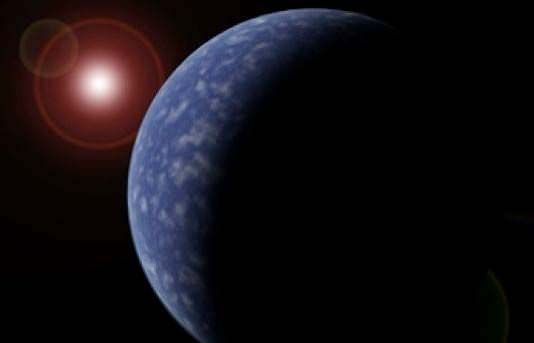
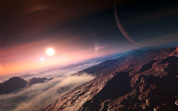
Artist's impression of a planet orbiting a red dwarf star. Credit: University of Hertfordshire
Good news for planet-hunters: planets around red dwarf stars are more abundant than previously believed, according to new research. A new study — which detected eight new planets around these stars — says that “virtually” all red dwarfs have planets around them. Moreover, super-Earths (planets that are slightly larger than our own) are orbiting in the habitable zone of about 25% of red dwarfs nearby Earth.
“We are clearly probing a highly abundant population of low-mass planets, and can readily expect to find many more in the near future – even around the very closest stars to the Sun,” stated Mikko Tuomi, who is from the University of Hertfordshire’s centre for astrophysics research and lead author of the study.
The find is exciting for astronomers as red dwarf stars make up about 75% of the universe’s stars, the study authors stated.
The researchers looked at data from two planet-hunting surveys: HARPS (High Accuracy Radial Velocity Planet Searcher) and UVES (Ultraviolet and Visual Echelle Spectrograph), which are both at the European Southern Observatory in Chile. The two instruments measure the effect a planet has on its parent star, specifically by examining the gravitational “wobble” the planet’s orbit produces.
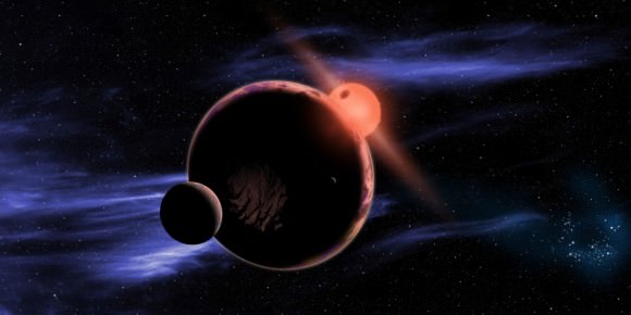
An artist’s concept of a rocky world orbiting a red dwarf star. (Credit: NASA/D. Aguilar/Harvard-Smithsonian center for Astrophysics).
Putting the information from both sets of data together, this amplified the planet “signals” and revealed eight planets around red dwarf stars, including three super-Earths in habitable zones. The researchers also applied a probability function to estimate how abundant planets are around this type of star.
The planets are between 15 and 80 light years away from Earth, and add to the 17 other planets found around low-mass dwarfs. Scientists also detected 10 weaker signals that could use more investigation, they said.
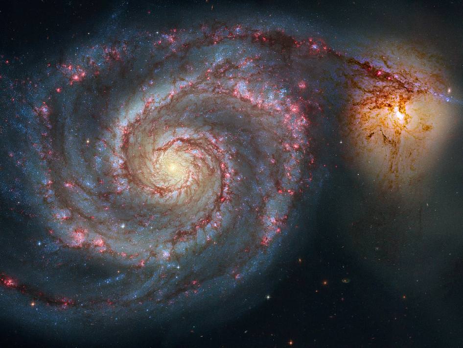
The 51st entry in Charles Messier's famous catalog is perhaps the original spiral nebula--a large galaxy with a well defined spiral structure also cataloged as NGC 5194. Over 60,000 light-years across, M51's spiral arms and dust lanes clearly sweep in front of its companion galaxy, NGC 5195. Image data from the Hubble's Advanced Camera for Surveys was reprocessed to produce this alternative portrait of the well-known interacting galaxy pair. The processing sharpened details and enhanced color and contrast in otherwise faint areas, bringing out dust lanes and extended streams that cross the small companion, along with features in the surroundings and core of M51 itself. The pair are about 31 million light-years distant. Not far on the sky from the handle of the Big Dipper, they officially lie within the boundaries of the small constellation Canes Venatici. Image Credit: NASA
The tangled remains of vast cosmic collisions can be seen across the universe, such as the distant Whirlpool Galaxy’s past close encounter with a nearby galaxy, which resulted in the staggering beauty we see today.
Such colossal collisions between galaxies appear to be common. It’s likely giant galaxies, such as our own, originated long ago after smaller dwarf galaxies crashed together. Unfortunately, Hubble has yet to peer into the early Universe and catch two dwarf galaxies merging by chance. And they’re extremely rare to catch in the present nearby universe.
But for the first time, astronomers have uncovered evidence of a similar collision much closer to home.
The Milky Way is part of a large cosmic neighborhood. A collection of more than 35 galaxies compose the Local Group. While the largest and heavier members are the Milky Way and the Andromeda galaxy, there are many smaller satellite galaxies orbiting the two. Anyone who has looked at the southern sky should be familiar with the Large and Small Magellanic Clouds: two satellite galaxies of the Milky Way less than 200,000 light years away.
Andromeda has over 20 satellite galaxies circling its nearly a trillion stars. A team of European astronomers has analyzed measurements of the stars in the dwarf galaxy Andromeda II — the second largest dwarf galaxy in the Local Group — and made a surprising discovery: an odd stream of stars that simply doesn’t belong.
The team led by Dr. Nicola C. Amorisco from the Dark Cosmology Centre at the Niels Bohr Institute in Copenhagen used the Deep Imaging Multi-Object (DEIMOS) spectrograph onboard the Keck II telescope in Hawaii in order to measure the velocities of more than 700 stars in the Andromeda II dwarf galaxy.
Stars in a large spiral galaxy will move, on average, with the rotation of the galaxy. On one side of the galaxy’s spinning disk, the stars will be moving away from the Earth, and their light waves will be stretched to redder wavelengths. On the opposite side, the stars will be moving toward the Earth, and their light waves will be compressed to bluer wavelengths.
But the stars in dwarf galaxies don’t exhibit such a pattern. Instead they move around entirely at random.
Amorisco and colleagues, however, found a rather different case present in Andromeda II. They observed a stream of stars — roughly 16,000 light years in length and 980 light years in thickness — that didn’t exhibit random motions at all. They orbit the center of the galaxy in a very coherent fashion.
But it gets better: the stars in this stream are also much colder than the stars outside the stream. In astronomy this is the equivalent of saying that the stars in this stream are much older. Amorisco’s team now believes they once belonged to a different galaxy entirely and remain only as a remnant of the past collision, which likely occurred over 3 billion years ago.
Streams of stars often result from collisions. As two galaxies begin to interact, the stars nearest the approaching galaxy feel a much stronger gravitational pull than the stars further away. Eventually the gravitational pull on the closer side of the galaxy will pull the stars from their initial galaxy, creating a stream of stars, dust and gas.
This is the smallest known example of two galaxies merging. The finding adds further evidence that mergers between dwarf galaxies plays a fundamental role in creating the large and beautiful galaxies we see today.
The paper has been published in Nature and is available for download here.
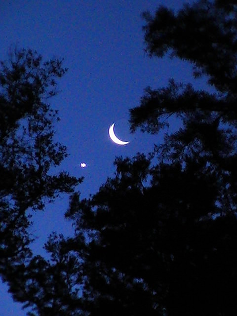
Did you see it? Earlier this week, we wrote about the spectacular conjunction of the planet Venus and the waning crescent Moon this week, which culminated in a fine occultation of the planet by our large natural satellite on Wednesday morning. The footprint of the occultation crossed northern Africa in the predawn hours to greet daytime observers across southern Asia. And although the pass was a near miss for many, viewers worldwide were treated to a fine photogenic pairing of Venus and the Moon.
An “aircraft/Moon/Venus tri-conjunction” captured February 26th from London, UK. Credit: Sculptor Lil
This was a highlight event of the 2014 dawn apparition of Venus, and some great pics have been pouring in to us here at Universe Today via Twitter, Google+ and our Flickr pool. We also learned a new word this week while immersed in astronomical research: a decrescent Moon. We first thought this was a typo when we came across it, but discovered that it stands for a waning crescent Moon going from Last Quarter phase to New. Hey, it’s got a great ring to it, and its less characters than “waning crescent” and thus comes ready Tweet-able.
Venus and the Moon in the predawn sky captured from Israel. Credit: Gadi Eidelheit @gadieid
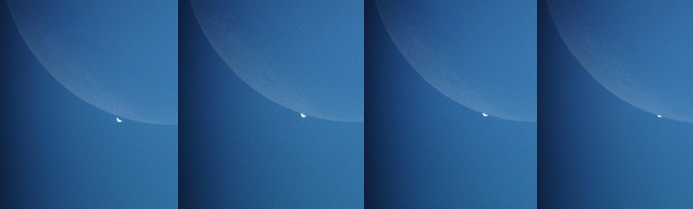
Some great video sequences have emerged as well, including this fine grazing sequence of a daytime crescent Venus brushing past the crescent Moon taken by Shahrin Ahmad:
Shahrin journeyed to the northern tip of Peninsular Malaysia to the town of Perlis near near the Thai border to capture the graze. “It was a really close event,” he noted. “Today, the clouds began to appear and posed some real tense moments during the occultation.”
And although many weren’t fortunate enough to be in the path of the occultation, many observers worldwide captured some very photogenic scenes of the conjunction between the Moon and Venus as the pair rose this morning, including this great video sequence from Ryan Durnall:
And clear skies greeted a series of early morning astronomers worldwide, who shared these amazing images with us:
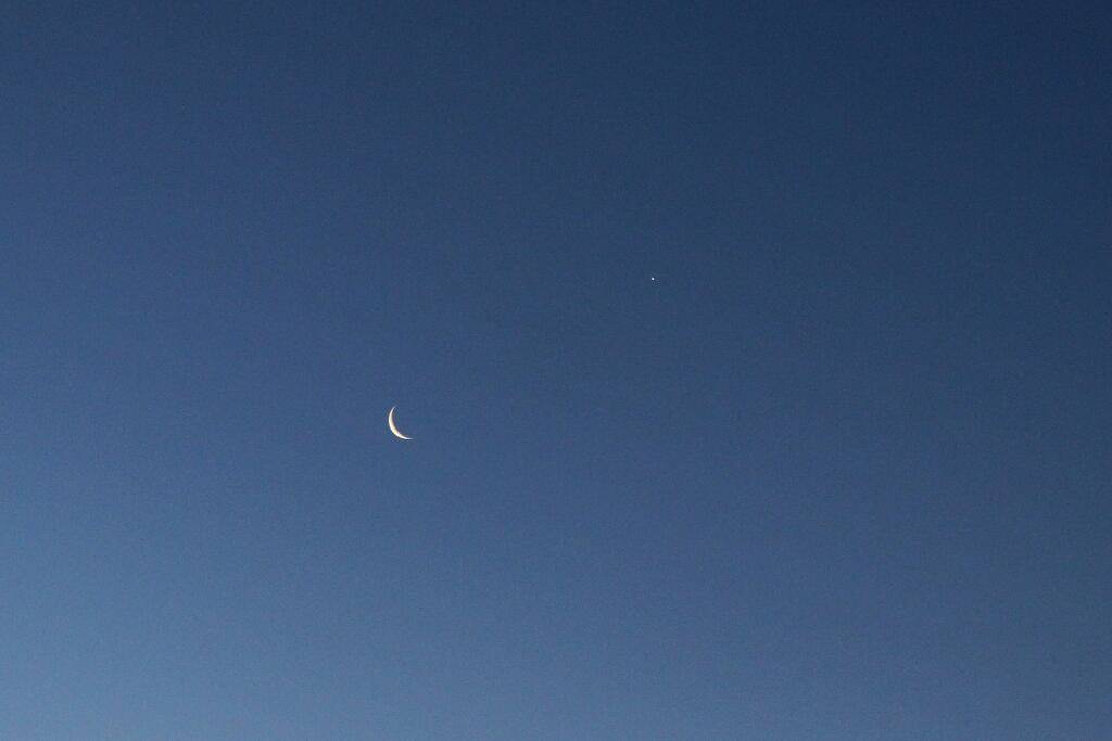
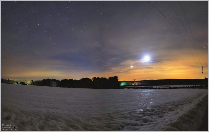
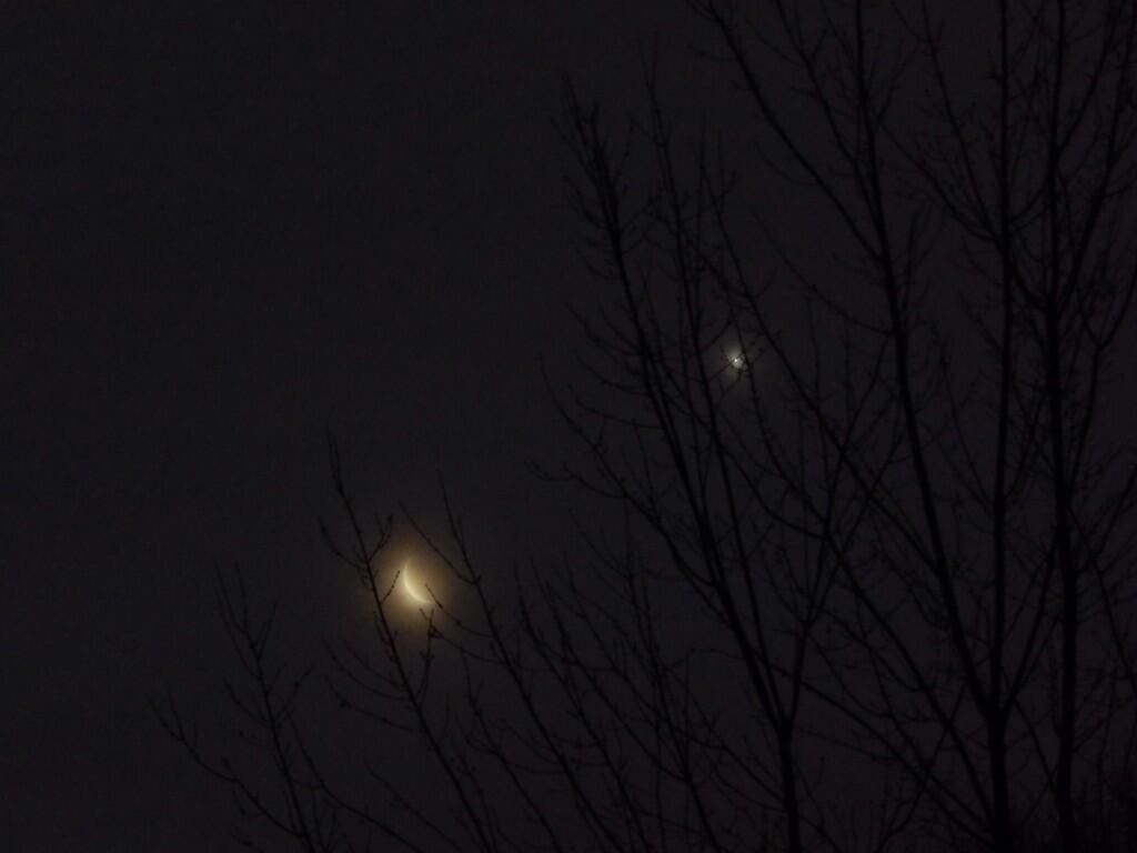
This morning’s conjunction as imaged from Newark, New York. Credit- Brad Timerson @btimersonVenus and the Moon the day prior to the occultation, shot by Ken Lord from Maple Ridge, British Columbia. Credit- Ken Lord.The Moon approaching Venus on February 25th as seen from Carbon County, Pennsylvania. Credit: Tom Wildoner.Venus and the Moon rising through the fog: Credit: Joanie Boloney @jstabila
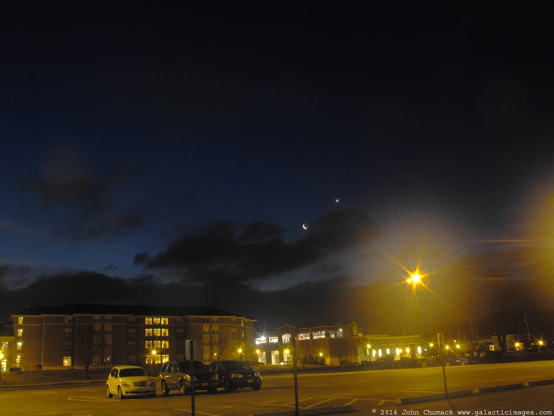
John Chumack was also up early this morning and was able to capture this fine image of the pair rising above the University of Dayton’s PAC Center:
Venus and the Moon as seen from Dayton, Ohio. Credit: John Chumack, www.galacticimages.com
“All I had available was a point and shoot camera (not even mine!)” Chumack told Universe Today. “I’m surprised it came out okay, considering all the ambient light on Campus!!!” Chumack used a Fujifilm Finepix S1000 point and shoot camera, and went sans tripod, doing a 2″ exposure with the camera perched atop a trash can. The results of this ad hoc setup look great!
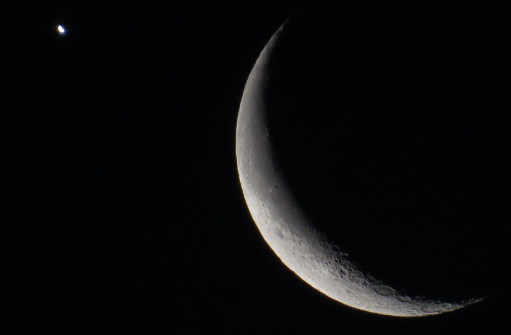
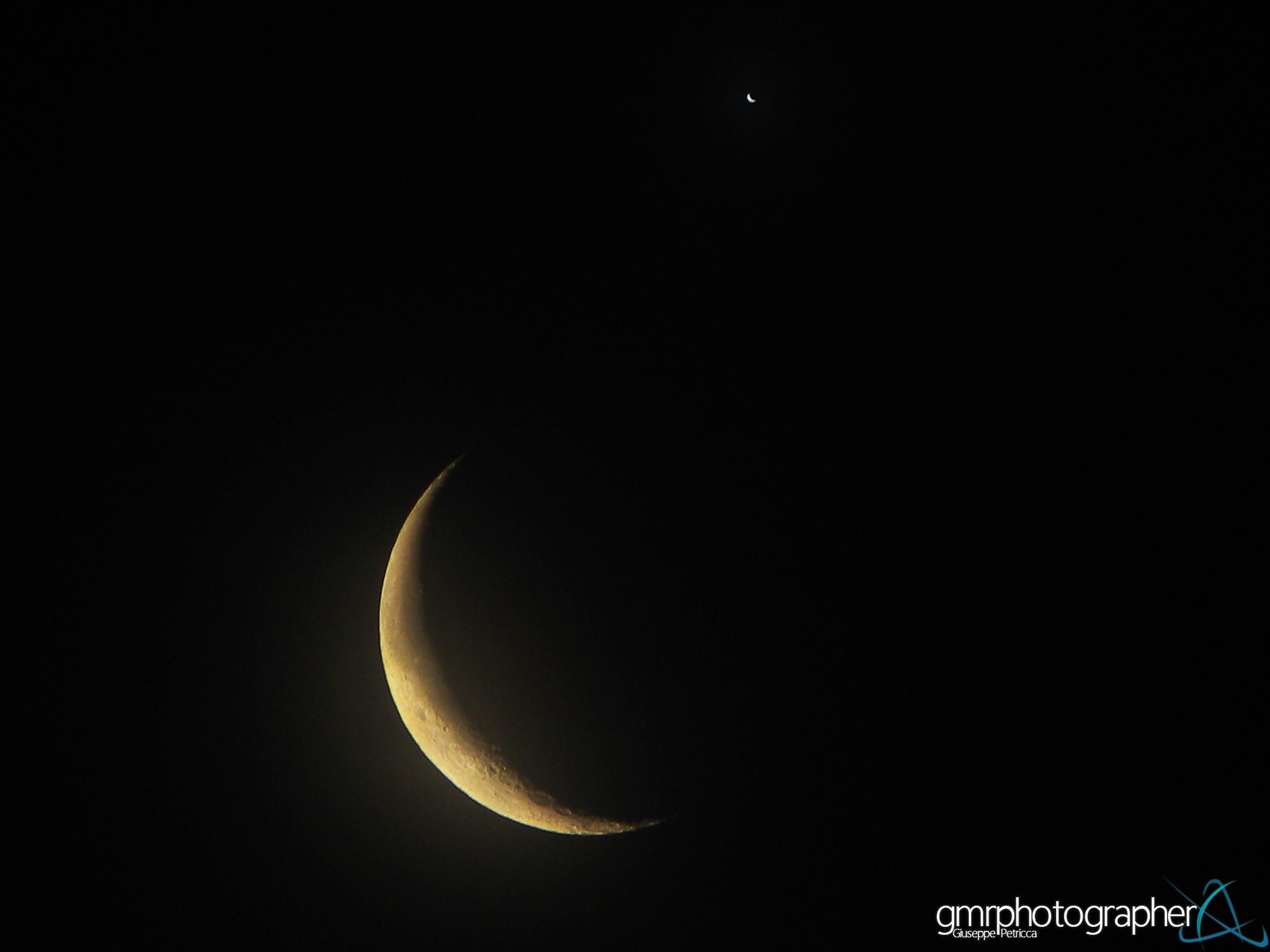
Astrophotographer Giuseppe Petricca based in Pisa, Italy north of the occultation path also grabbed this outstanding closeup image of the crescent pair:
Taken using a Nikon Coolpix P90 Bridge camera on a tripod mount. Credit: Giuseppe Petricca
“This morning was awesome!” Petricca told Universe Today. “The weather forecast showed a compact high layer of clouds, but there were enough gaps between them that allowed me to see the conjunction in a lot of different moments.”
You can compare and contrast the twin crescents of Venus and the Moon evident in the above image. “You can easily see the phase of the Planet Venus and a lot of details on the lunar surface, despite the high clouds that partially blocked the view sometimes!” Petricca noted.
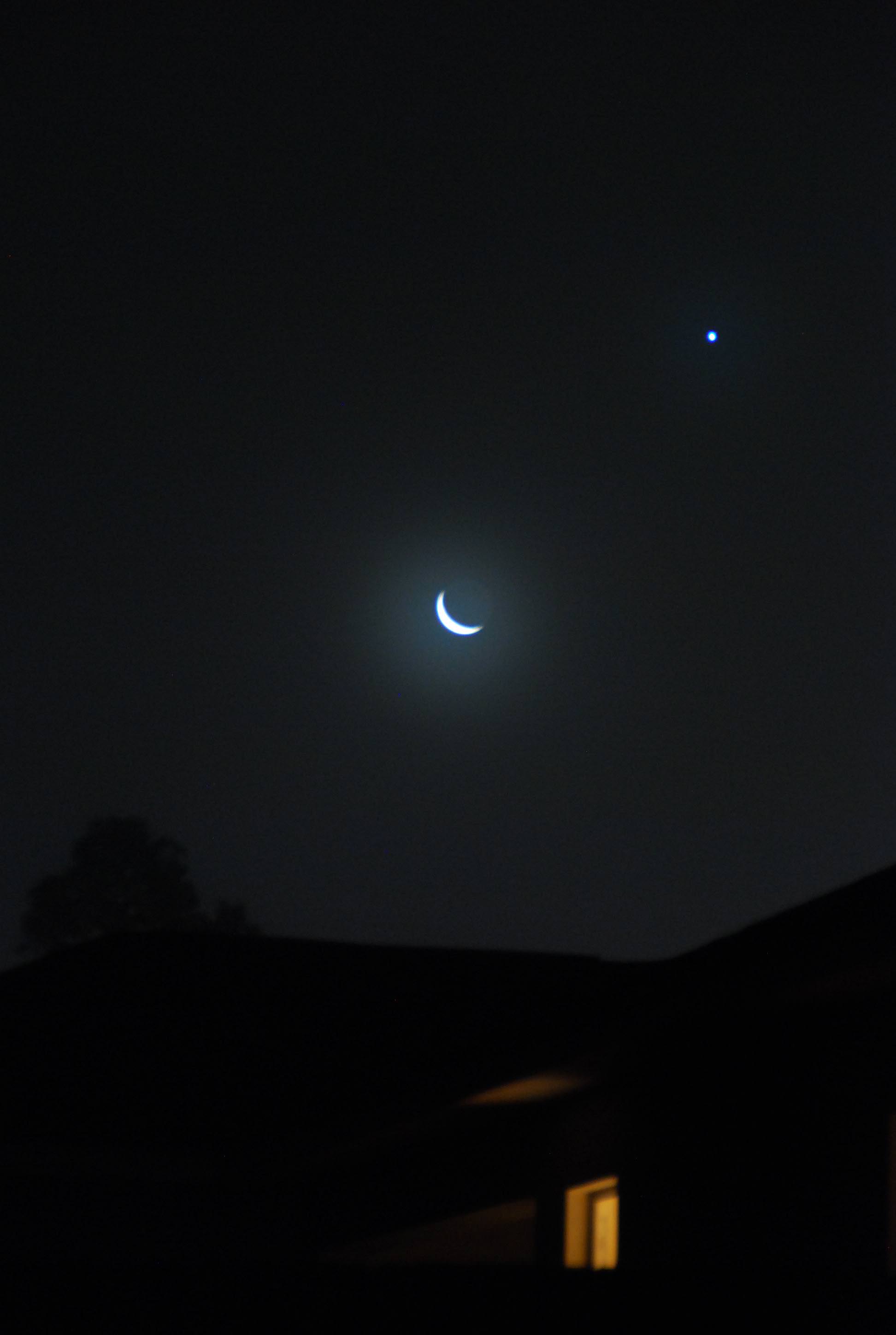
And finally, I give you our own humble entry, a conjunction over suburbia snapped pre-caffeination:
We think its great that you can sometimes catch a memorable glimpse of the celestial even from your own doorstep.
And when is the next occultation of a planet by the Moon? That would be next month, when Saturn is occulted by the waxing gibbous Moon for South Africa and Brazil after sunset on March 21st, 2014. We’re in the midst of a cycle of occultations of the ringed planet by the Moon, occurring every lunation through the final one this year on October 25th.
The next occultation of Venus occurs on October 23rd 2014, but is only one degree from the Sun and is unobservable. The next observable event occurs on July 19th 2015 for northern Australia in the daytime, and for a remote stretch of the South Pacific at dusk.
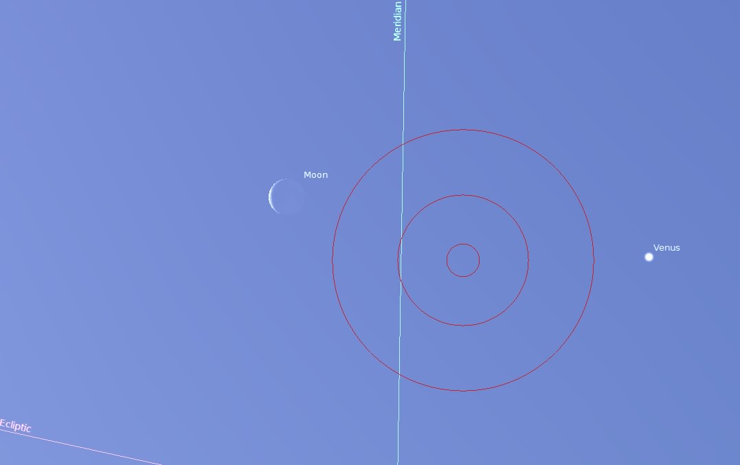
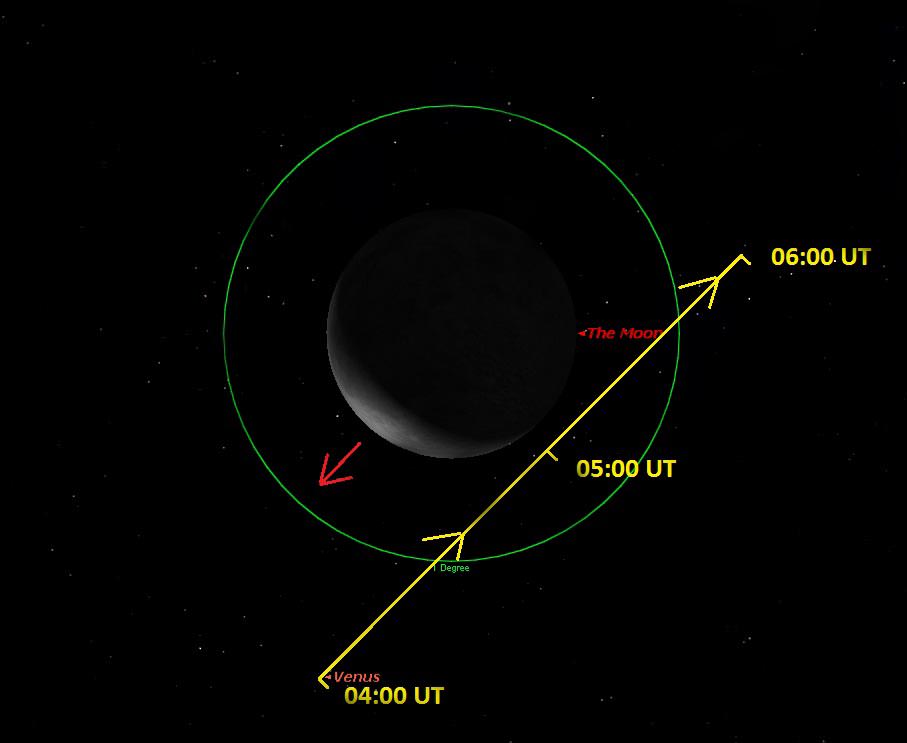
And its still not too late to spy Venus in the daytime today, using the nearby Moon as a guide. Here’s a handy simulation to aid you in your quest generated for mid-noon, February 26th:
The orientation of the Moon and Venus at ~17:00UT, including a five degree Telrad bullseye. Created by the author using Stellarium.
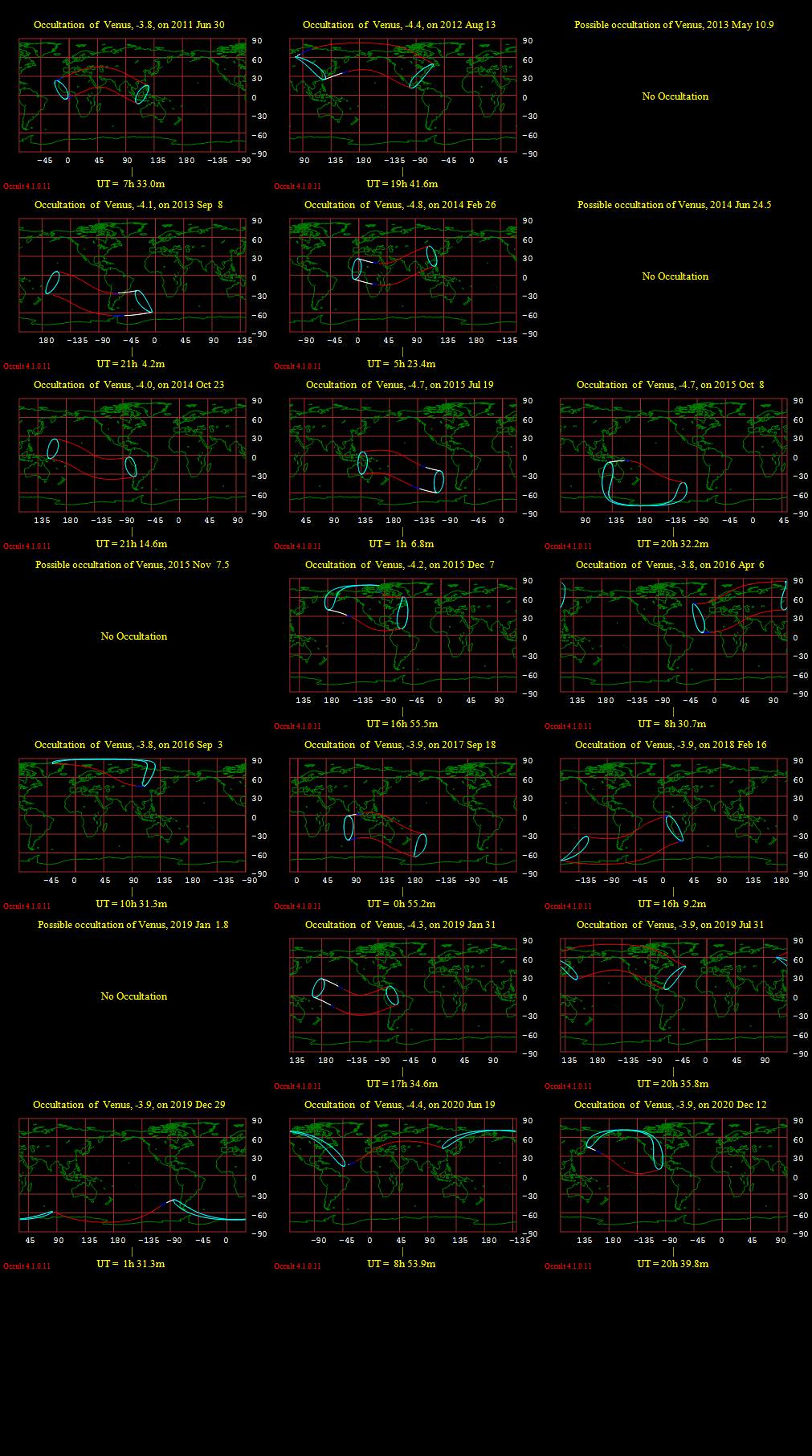
And finally here’s handy chart of maps of occultations of Venus by the Moon for the current decade, just click to enlarge:
Occultations of Venus by the Moon from 2011-2020. Created using Occult 4.0.
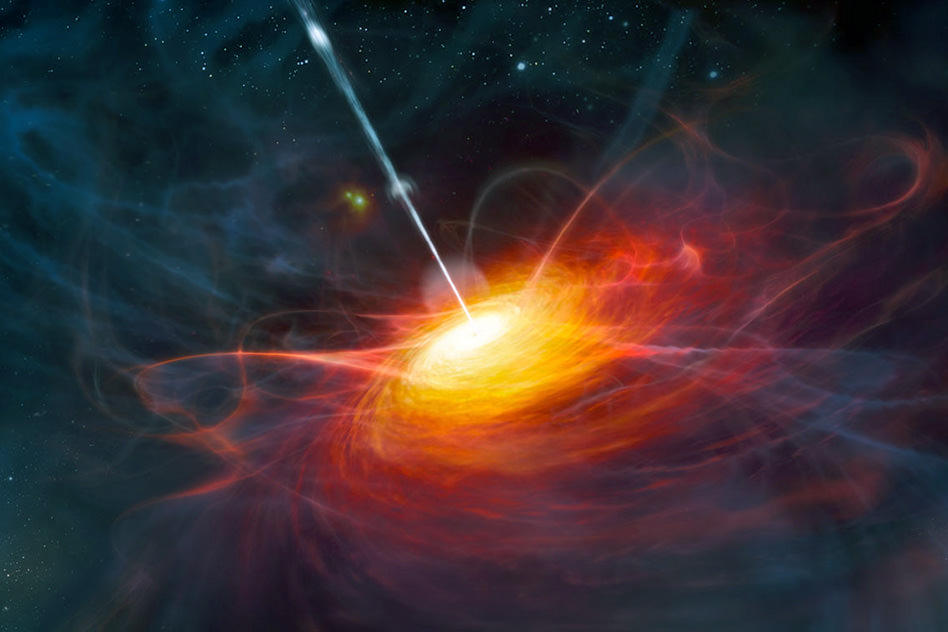
Artist’s interpretation of ULAS J1120+0641, a very distant quasar with a supermassive black hole at its heart.
Credit: ESO/M. Kornmesser
Do you believe in free will? Are people able to decide their own destinies, whether it’s on what continent they’ll live, who or if they’ll marry, or just where they’ll get lunch today? Or are we just the unwitting pawns of some greater cosmic mechanism at work, ticking away the seconds and steering everyone and everything toward an inevitable, predetermined fate?
Philosophical debates aside, MIT researchers are actually looking to move past this age-old argument in their experiments once and for all, using some of the most distant and brilliant objects in the Universe.
Rather than ponder the ancient musings of Plato and Aristotle, researchers at MIT were trying to determine how to get past a more recent conundrum in physics: Bell’s Theorem. Proposed by Irish physicist John Bell in 1964, the principle attempts to come to terms with the behavior of “entangled” quantum particles separated by great distances but somehow affected simultaneously and instantaneously by the measurement of one or the other — previously referred to by Einstein as “spooky action at a distance.”
The problem with such spookiness in the quantum universe is that it seems to violate some very basic tenets of what we know about the macroscopic universe, such as information traveling faster than light. (A big no-no in physics.)
(Note: actual information is not transferred via quantum entanglement, but rather it’s the transfer of state between particles that can occur at thousands of times the speed of light.)
Then again, testing against Bell’s Theorem has resulted in its own weirdness (even as quantum research goes.) While some of the intrinsic “loopholes” in Bell’s Theorem have been sealed up, one odd suggestion remains on the table: what if a quantum-induced absence of free will (i.e., hidden variables) is conspiring to affect how researchers calibrate their detectors and collect data, somehow steering them toward a conclusion biased against classical physics?
“It sounds creepy, but people realized that’s a logical possibility that hasn’t been closed yet,” said David Kaiser, Germeshausen Professor of the History of Science and senior lecturer in the Department of Physics at MIT in Cambridge, Mass. “Before we make the leap to say the equations of quantum theory tell us the world is inescapably crazy and bizarre, have we closed every conceivable logical loophole, even if they may not seem plausible in the world we know today?”
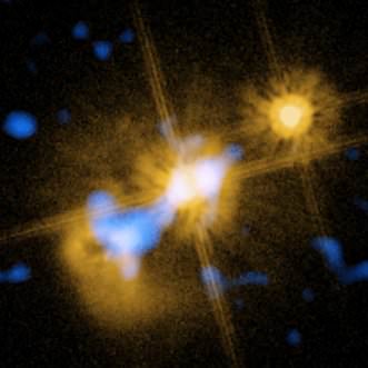
A color composite image of the quasar in HE0450-2958 obtained using the VISIR instrument on the Very Large Telescope and the Hubble Space Telescope. Image Credit: ESO
So in order to clear the air of any possible predestination by entangled interlopers, Kaiser and MIT postdoc Andrew Friedman, along with Jason Gallicchio of the University of Chicago, propose to look into the distant, early Universe for sufficiently unprejudiced parties: ancient quasars that have never, ever been in contact.
…an experiment would go something like this: A laboratory setup would consist of a particle generator, such as a radioactive atom that spits out pairs of entangled particles. One detector measures a property of particle A, while another detector does the same for particle B. A split second after the particles are generated, but just before the detectors are set, scientists would use telescopic observations of distant quasars to determine which properties each detector will measure of a respective particle. In other words, quasar A determines the settings to detect particle A, and quasar B sets the detector for particle B.
By using the light from objects that came into existence just shortly after the Big Bang to calibrate their detectors, the team hopes to remove any possibility of entanglement… and determine what’s really in charge of the Universe.
“I think it’s fair to say this is the final frontier, logically speaking, that stands between this enormously impressive accumulated experimental evidence and the interpretation of that evidence saying the world is governed by quantum mechanics,” said Kaiser.
Then again, perhaps that’s exactly what they’re supposed to do…
The paper was published this week in the journal Physical Review Letters.
Want to read more about the admittedly complex subject of entanglement and hidden variables (which may or may not really have anything to do with where you eat lunch?) Click here.
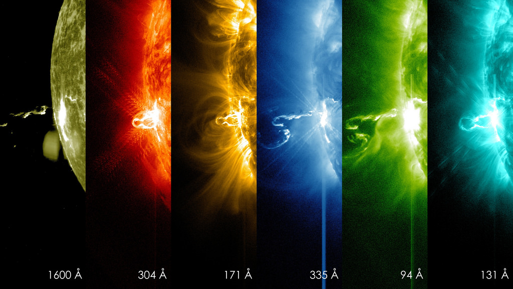
NASA's Solar Dynamics Observatory captured these images of a large flare erupting from the sun Feb. 21, 2014. Credit: NASA/SDO
She’s a rainbow! You can see the first moments of a huge flare belching off the sun in the picture above. The so-called X-class flare erupted a few hours ago (at 7:25 p.m. EST Feb. 24, or 12:25 a.m. UTC Feb. 25) and was captured by several spacecraft. If you have a pictures of the sun yourself to share, feel free to post them in the Universe Today Flickr pool.
NASA’s Solar Dynamics Observatory saw the flare growing in at least six different wavelengths of light, which are visible in the image above. This is classified this as an X4.9-class flare, which shows that it is pretty strong. X-flares are the most powerful kind that the sun emits, and each X number is supposed to be twice as intense as the previous one (so an X-2 flare is twice as powerful as X-1, for example).
SpaceWeather.com says this is the most powerful flare of the year so far, emitted from sunspot AR1967 (or more properly speaking, AR1990; sunspots are renamed if they survive a full rotation of the sun, as this one has done twice already!) While solar flares can lead to auroras, in this case it appears the blast was pointed in the wrong direction, the site added.
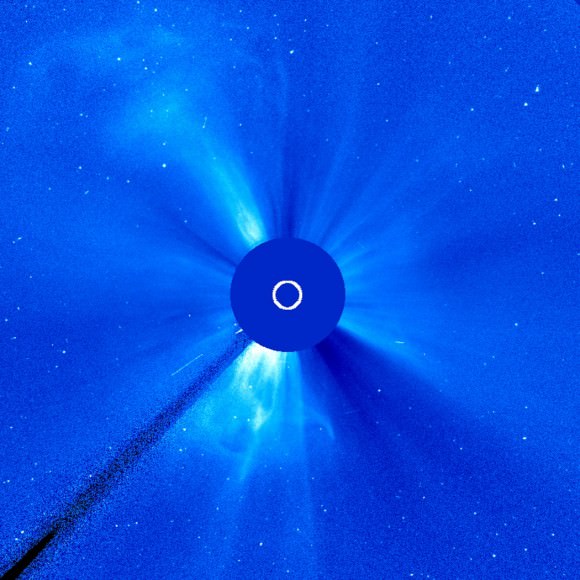
“Although this flare is impressive, its effects are mitigated by the location of the blast site–near the sun’s southeastern limb, and not facing Earth,” SpaceWeather stated. “Indeed, a bright coronal mass ejection (CME) which raced away from the sun shortly after the flare appears set to miss our planet.”
This image from the Solar and Heliospheric Observatory illustrates increased solar activity between Feb. 18-20, 2014. Credit: ESA/NASA/SOHO/GSFC
The sun goes through an 11-year cycle of sunspot and solar activity, which is supposed to be at its peak right now. This particular peak has been very muted, but lately things have been picking up. The European Space Agency noted that between Feb. 18 and 20, the sun sent out six CMEs in three days, with most of them moving in different directions.
“This level of activity is consistent with what we might expect as the Sun is near its maximum period of activity in the 11-year solar cycle,” ESA stated.
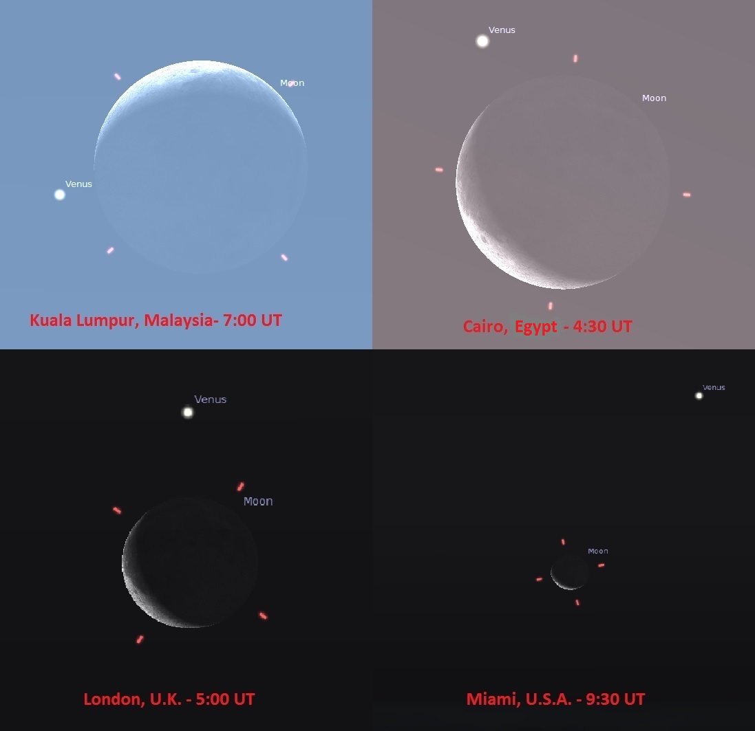
The view of Wednesday's conjunction from selected sites based on four separate continents. Credit: Created by the author using Stellarium.
Are you ready for some lunar versus planetary occultation action? One of the best events for 2014 occurs early this Wednesday morning on February 26th, when the waning crescent Moon — sometimes referred to as a decrescent Moon — meets up with a brilliant Venus in the dawn sky. This will be a showcase event for the ongoing 2014 dawn apparition of Venus that we wrote about recently.
This is one of 16 occultations of a planet by our Moon for 2014, which will hide every naked eye classical planet except Jupiter and only one of two involving Venus this year.
An occultation occurs when one celestial body passes in front of another, obscuring it from our line of sight. The term is used to refer to planets or asteroids blocking out distant stars or the Moon passing in front of stars or planets.
Wednesday’s event has a central conjunction time of 5:00 Universal. Viewers in northwestern Africa based in Mali and southern Algeria and surrounding nations will see the occultation occur in the dawn sky before sunrise, while viewers eastward across the Horn of Africa, the southern Arabian peninsula, India and southeast Asia will see the occultation occur in the daylight.
A comparison of Venus versus the Moon in the daytime taken by Sharin Ahmad (@shahgazer) from Malaysia during the last lunation on January 29th, 2014.
Observers worldwide, including those based in Australia, Europe and the Americas will see a near miss, but early risers will still be rewarded with a brilliant dawn pairing of the second and third brightest objects in the night sky. This will also be a fine time to attempt to spot Venus in the daytime, using the nearby crescent Moon as a guide. It’s easier than you might think! In fact, Venus is actually brighter than the Moon per apparent square arc second of surface area, owing to its higher average reflectivity (known as albedo) of 80% versus the Moon’s dusky 14%.
The International Occultation Timing Association also maintains a chart of ingress and egress times for specific locations along the track of the occultation.
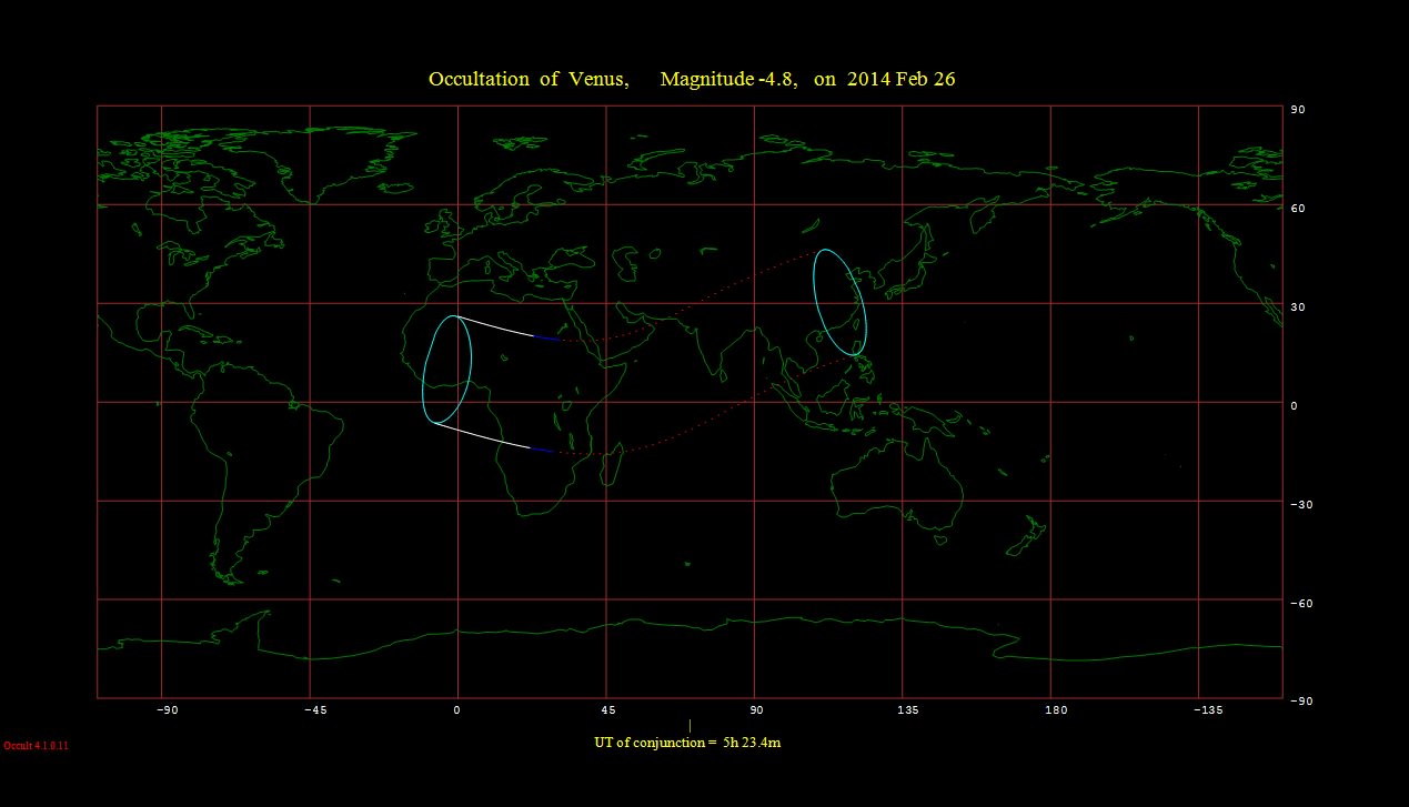
The footprint of the Wednesday occultation of Venus by the Moon. Solid lines indicate where the occultation occurs before sunrise, while the dashed area denotes where the occultation occurs after sunrise. Credit: Created using Occult4.1.0.11.
The Moon occults Venus 21 times in this decade. The last occultation of Venus by the Moon occurred on September 8th, 2013, and the next occurs October 23rd 2014 over the South Pacific in daylight skies very close to the Sun, and is unobservable.
Wednesday’s event also offers a unique opportunity to catch a crescent Venus emerging from behind the dark limb of the Moon. On Wednesday, Venus presents a 34” diameter disk that is 35% illuminated and shining at magnitude -4.3, while the Moon is a 12% illuminated crescent three days from New. Fun fact: February 2014 is missing a New Moon, meaning that both January and March will each contain two!
Apparent path of Venus in relation to the Moon Wednesday morning as seen from a theoretical geocentric (Earth-centered) location. Created using Starry Night Education software.
This also means that a well positioned observer in northwestern Africa would be able to see able to catch the dark limb of Venus creeping out from behind the nighttime side of the Moon against a dark sky. Such favorable occurrences only happen a handful of times per decade, and this week would be a great time to try and briefly spot – or perhaps even video or photograph – a phenomenon know as the ashen light of Venus as the dazzling crescent daytime side of the planet lay obscured by the Moon. Is this effect reported by observers over the years a fanciful illusion, or a real occurrence?
Perhaps, due to the remote location, this chance to spy and record this elusive effect will go unnoticed this time ‘round. The next chance with optimal possibilities to catch a crescent Venus occulted by the Moon against a dark sky occurs next year on October 8th, 2015, favoring the Australian outback. Anyone out there down for an observing expedition to prove or disprove the ashen light of Venus once and for all? Astronomy road trip!
April 22nd, 2009 conjunction of Venus and the Moon as seen from Hudson, Florida. The Photo by author.
This event also provides optimal circumstances as Venus heads towards greatest elongation west of the Sun on March 22nd and the Moon-Venus pair lay 43 degrees west of the Sun during Wednesday’s event. Compare this to the impossible to observe occultation this October, when the pairing is only one degree east of the Sun! The next occultation of Venus for North America occurs next year on December 7th, 2015 and will be visible in the daytime across the extent of the track except for Alaska and Northwestern Canada.
Vexillographers may also want to take note: this week’s Venus-Moon pairing will closely emulate the familiar crescent Moon plus star pairing seen on many national flags worldwide. Did an ancient and unrecorded occultation of Venus by the Moon inspire this meme? Tradition has it that Sultan Alp Arslan settled on the star and crescent for the flag of the Turks after witnessing a close conjunction after the defeat of the Byzantine Army at the Battle of Manzikert on August 26th, 1071 A.D. This tale, however, is almost certainly apocryphal, as no occultations of planets or bright stars by the Moon occurred on or near that date, and only two occultations of Venus by the Moon occurred that year. And Venus was less than two degrees from the Sun on that date, yet another strike against it. In fact, the only occultations of Venus by the Moon in 1071 occurred on June 29th and November 27th. Perhaps Arslan just took a while to decide…
Still, this week’s event provides a great photo-op to have “Fun with Flags” and capture the pair behind your favorite astronomical conjunction-depicting banner. And be sure to send those pics into Universe Today… methinks there’s a good chance of us running a post occultation photo-essay later this week!
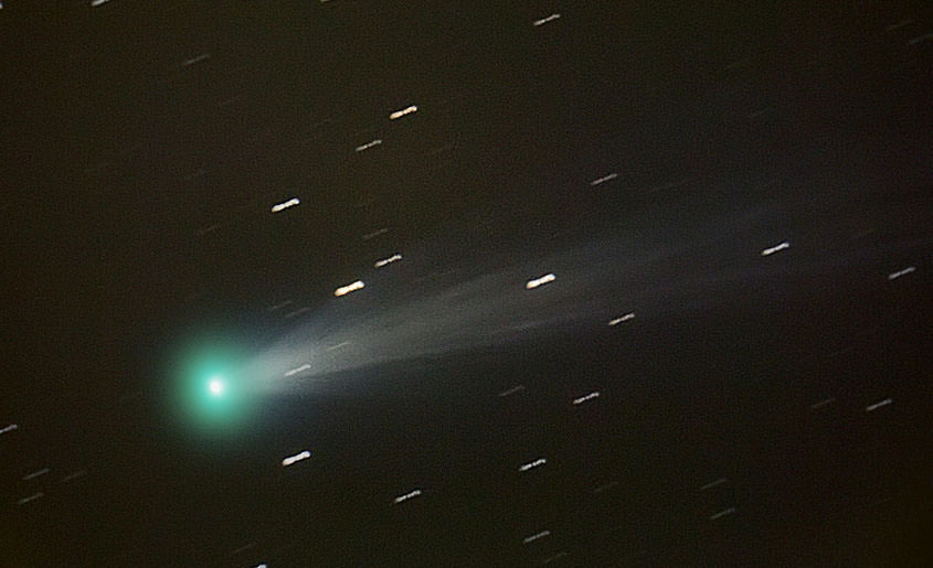
Spectacular photo of Comet ISON taken Nov. 15 from Charleston, Rhode Island, USA showing the recent outburst. Click to enlarge. Credit: Scott MacNeill
Comet ISON — that bright comet last year that broke up around Thanksgiving weekend — included two forms of nitrogen in its icy body, according to newly released observations from the Subaru Telescope.
Of the two types found, the discovery of isotope 15NH2 was the first time it’s ever been seen in a comet. Further, the observations from the Japanese team of astronomers show “there were two distinct reservoirs of nitrogen [in] the massive, dense cloud … from which our Solar System may have formed and evolved,” stated the National Astronomical Observatory of Japan.
Besides being pretty objects to look at, comets are considered valuable astronomical objects because they’re a sort of time capsule of conditions early in the universe. The “fresh” comets are believed to come from a vast area of icy bodies called the Oort Cloud, a spot that has been relatively untouched since the solar system formed about 4.6 billion years ago. Spying elements inside of comets can give clues as to what was present in our neighborhood when the sun and planets were just coming to be.
“Ammonia (NH3) is a particularly important molecule, because it is the most abundant nitrogen-bearing volatile (a substance that vaporizes) in cometary ice and one of the simplest molecules in an amino group (–NH2) closely related to life. This means that these different forms of nitrogen could link the components of interstellar space to life on Earth as we know it,” NAOJ stated.
You can read more details about the finding at the NAOJ website, or in Astrophysical Journal Letters.
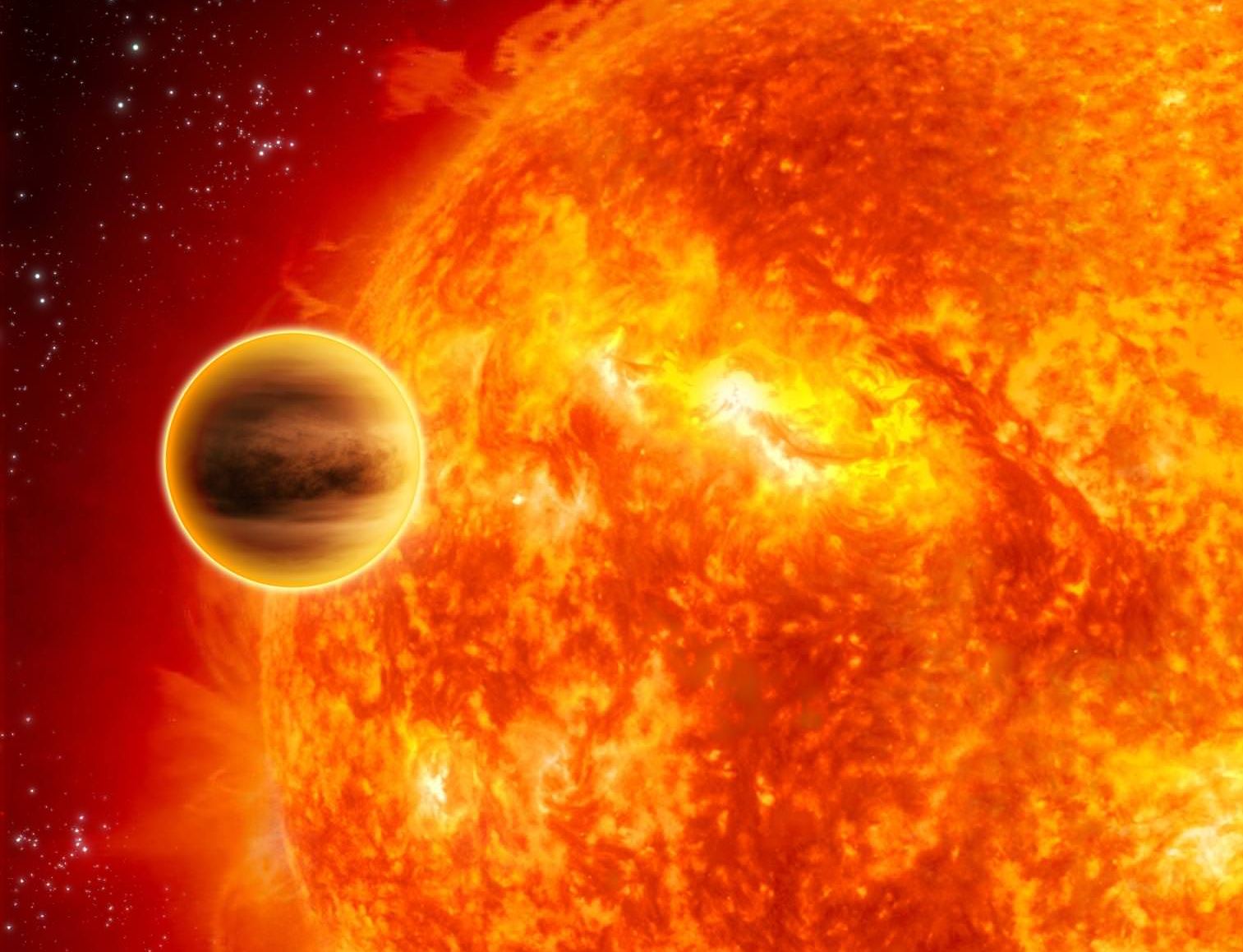
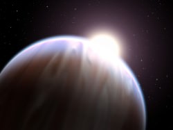
An exoplanet transiting across the face of its star, demonstrating one of the methods used to find planets beyond our solar system. Credit: ESA/C. Carreau
With exoplanet discoveries coming at us several times a month, finding these worlds is a hot field of research. Once the planets are found and confirmed, however, there’s a lot more that has to be done to understand them. What are they made of? How habitable are they? What are their atmospheres like? These are questions we are only beginning to understand.
One long-standing exoplanet researcher argues that we don’t know very much about about alien planet atmospheres, as an example. Princeton University’s Adam Burrows says that not only is our understanding at an infancy, but the media and scientists overhype information based on very little data.
“Exoplanet research is in a period of productive fermentation that implies we’re doing something new that will indeed mature,” Burrows stated in a story posted on Princeton Journal Watch. “Our observations just aren’t yet of a quality that is good enough to draw the conclusions we want to draw.”
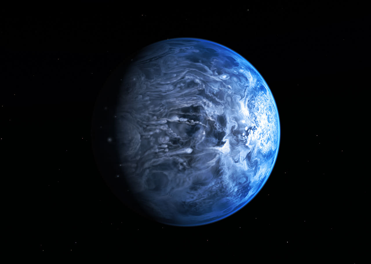
Artist’s conception of HD 189733 b, which may have winds that blow up to 22,000 mph (35,000 km/h). Credit: NASA
Burrow’s skepticism comes from how information on exoplanet atmospheres is collected. That uses a method called low-resolution photometry, which shows changes in light and radiation emitted from an object such as a planet. This could be affected by things such as a planet’s rotation and cloud cover.
Burrows’ solution is to use spectrometry, which can glean physical information through looking at light spectra, but that would be a challenge given the existing exoplanet-seeking infrastructure in space and on Earth uses telescopes that generally rely on other methods.
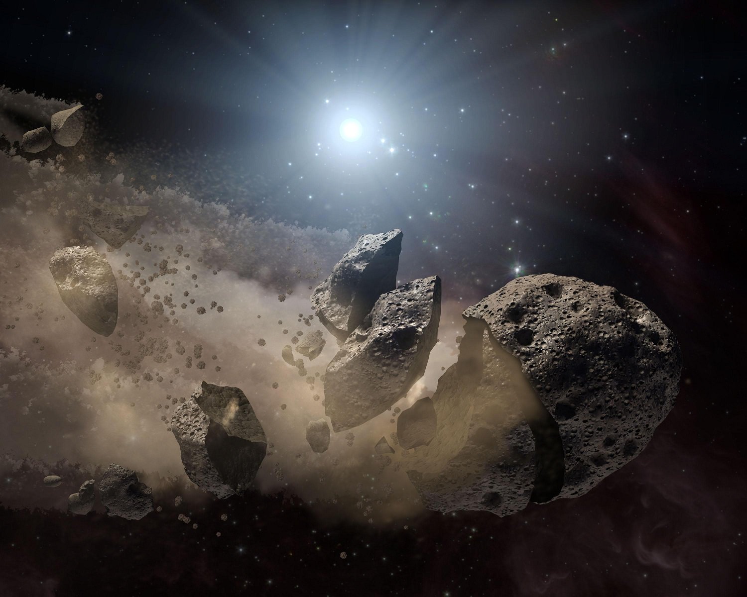
Artist's impression of an asteroid breaking up. Credit: NASA/JPL-Caltech
When you throw a bunch of rock and debris at a rapidly spinning star, what happens? A new study suggests that so-called pulsar stars change their dizzying spin rate as asteroids fall into the gaseous mass. This conclusion comes from observations of one pulsar (PSR J0738-4042) that is being “pounded” with debris from rocks, researchers said.
Lying 37,000 light-years from our planet in the southern constellation Puppis, this supernova remnant’s environment is swarming with rocks, radiation and “winds of particles”. One of those rocks likely was more than a billion metric tonnes in mass, which is nowhere near the mass of Earth (5.9 sextillion tonnes), but is still substantial.
“If a large rocky object can form here, planets could form around any star. That’s exciting,” stated Ryan Shannon, a researcher with the Commonwealth Scientific and Industrial Research Organisation who participated in the study.
Pulsars are sometimes called the clocks of the universe because their spins, fast as they are, precisely emit radio beams with each revolution — a beam that can be seen from Earth if our planet and the star are aligned in the right way. A 2008 study by Shannon and others predicted the spin could be altered by debris falling into the pulsar, which this new research appears to confirm.
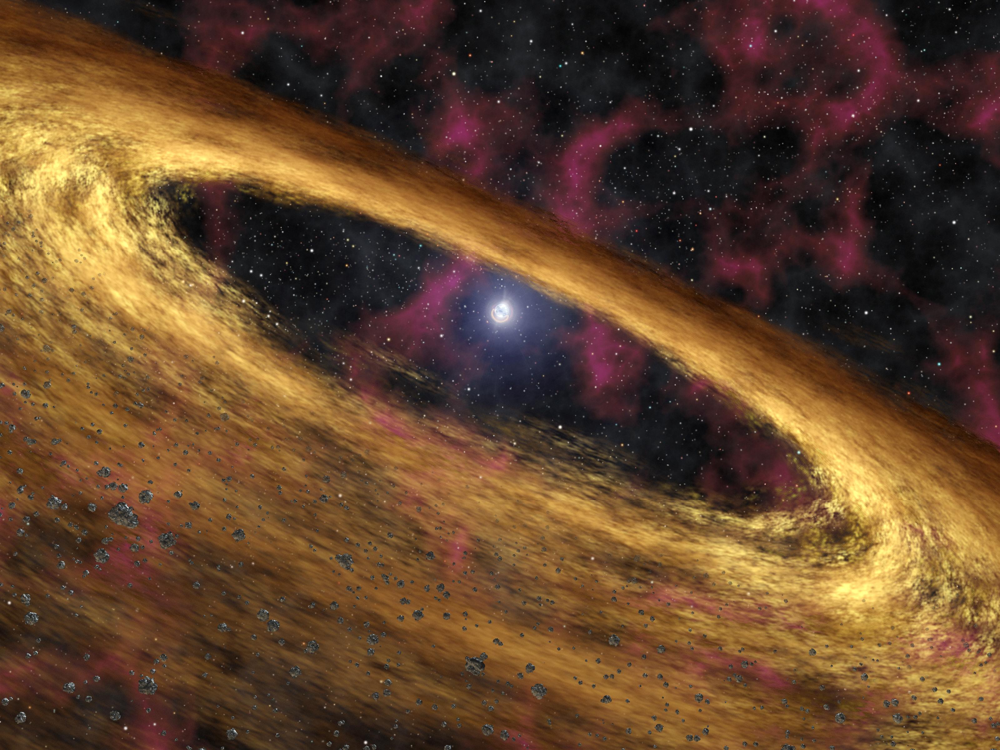
Artist’s conception of stellar rubble around pulsar 4U 0142+61. Credit: NASA/JPL-Caltech
“We think the pulsar’s radio beam zaps the asteroid, vaporizing it. But the vaporized particles are electrically charged and they slightly alter the process that creates the pulsar’s beam,” Shannon said.
As stars explode, the researchers further suggest that not only do they leave behind a pulsar star remnant, but they also throw out debris that could then fall back towards the pulsar and create a debris disc. Another pulsar, J0146+61, appears to display this kind of disc. As with other protoplanetary systems, it’s possible the small bits of matter could gradually clump together to form bigger rocks.
You can read the study in Astrophysical Journal Letters or in preprint version on Arxiv. The study was led by Paul Brook, a Ph.D. student co-supervised by the University of Oxford and CSIRO. Observations were performed with the Hartebeesthoek Radio Astronomy Observatory in South Africa, and CSIRO’s Parkes radio telescope.
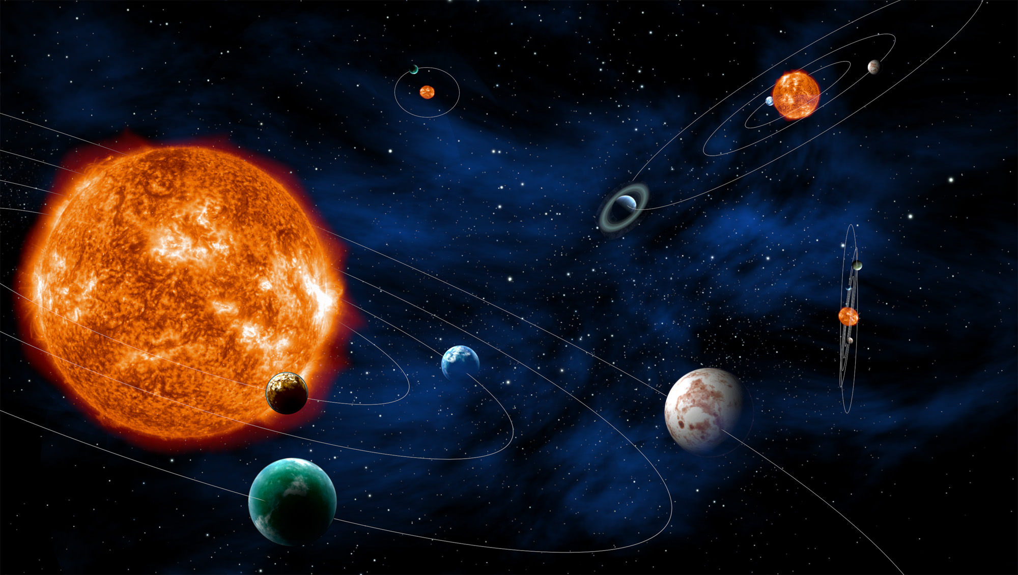
Artist's conception of exoplanet systems that could be observed by PLAnetary Transits and Oscillations of stars (PLATO), a European Space Agency telescope. Credit: ESA - C. Carreau
How could life arise in young solar systems? We’re still not sure of the answer on Earth, even for something as basic as if water arose natively on our planet or was carried in from other locations. Seeking answers to life’s beginnings will require eyes in the sky and on the ground looking for alien worlds like our own. And just yesterday, the European Space Agency announced it is going to add to that search.
The newly selected mission is called PLATO, for Planetary Transits and Oscillations. Like NASA’s Kepler space telescope, PLATO will scan the sky in search of stars that have small, periodic dips in their brightness that happen when planets go across their parent star’s face.
“The mission will address two key themes of Cosmic Vision: what are the conditions for planet formation and the emergence of life, and how does the solar system work,” stated ESA, referring to its plan for space science missions that extends from 2015 to 2025.
An exoplanet seen from its moon (artist’s impression). Via the IAU.
PLATO will operate far from Earth in a spot known as L2, a relatively stable Lagrange point about 1.5 million kilometers (930,000 miles) away from Earth in the opposite direction from the sun. Sitting there for at least six years, the observatory (which is actually made up of 34 small telescopes and cameras) will examine up to a million stars across half of the sky.
Find “statistically significant” Earth-mass planets in the habitable regions of several kinds of main-sequence stars;
Figure out the radius and mass of the star and any planets with 1% accuracy, and estimate the age of exoplanet systems with 10% accuracy;
Better determine the parameters of different kinds of planets, ranging from brown dwarfs (failed stars) to gas giants to rocky planets, all the way down to those that are smaller than Earth.
Artist’s impression of the deep blue planet HD 189733b, based on observations from the Hubble Space Telescope. Credit: NASA/ESA.
Adding PLATO’s observations to those telescopes on the ground that look at the radial velocity of planets, researchers will also be able to figure out each planet’s mass and radius (which then leads to density calculations, showing if it is made of rock, gas, or something else).
“The mission will identify and study thousands of exoplanetary systems, with an emphasis on discovering and characterising Earth-sized planets and super-Earths in the habitable zone of their parent star – the distance from the star where liquid surface water could exist,” ESA stated this week.
The telescope was selected from four competing proposals, which were EChO (the Exoplanet CHaracterisation Observatory), LOFT (the Large Observatory For x-ray Timing), MarcoPolo-R (to collect and return a sample from a near-Earth asteroid) and STE-Quest (Space-Time Explorer and QUantum Equivalence principle Space Test).
You can read more about PLATO at this website. It’s expected to launch from Kourou, French Guiana on a Soyuz rocket in 2024, with a budget of 600 million Euros ($822 million). And here’s more information on the Cosmic Vision and the two other M-class missions launching in future years, Euclid and Solar Orbiter.