On the Road to One Thousand Exoplanets

Planets everywhere. So where are all the aliens? Credit: ESO/M. Kornmesser

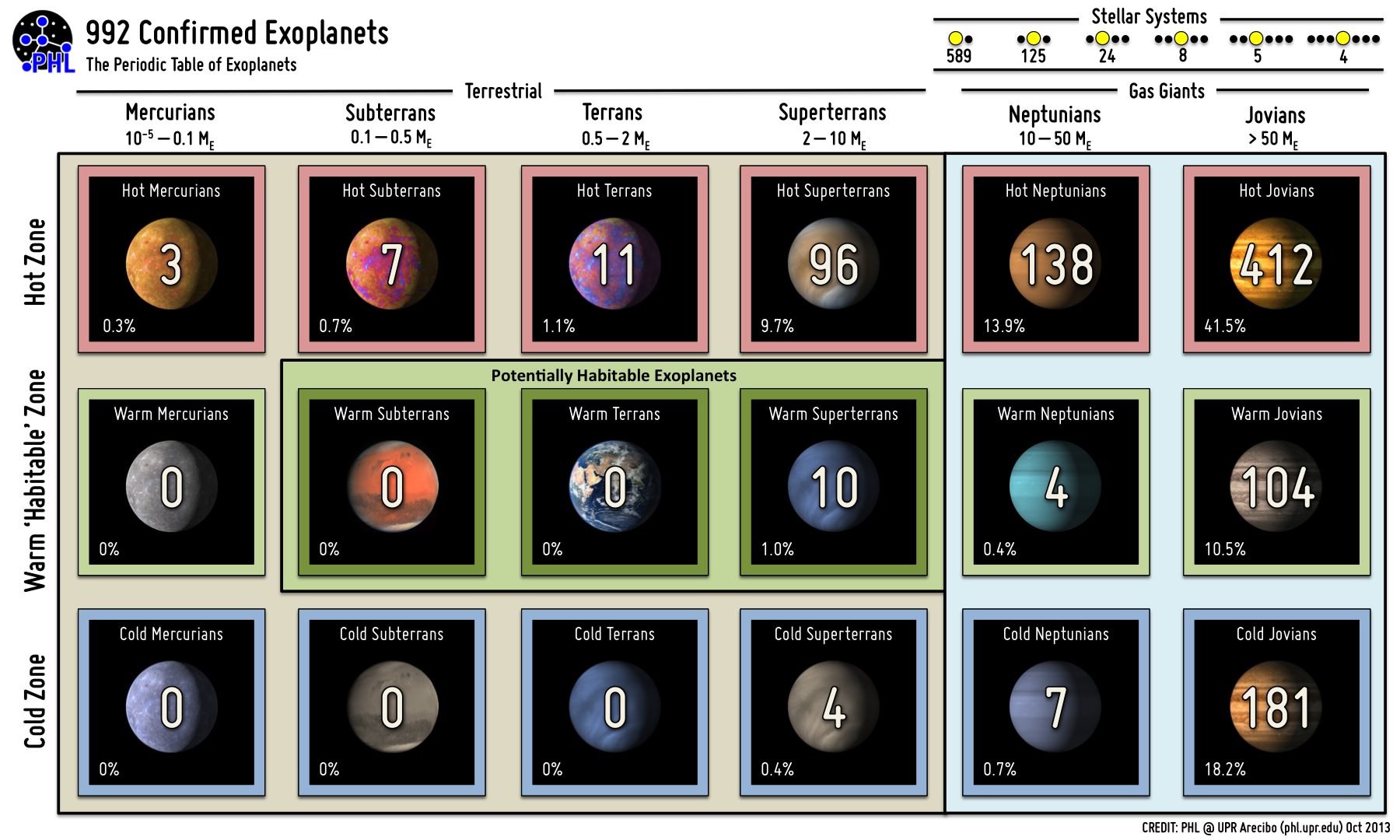
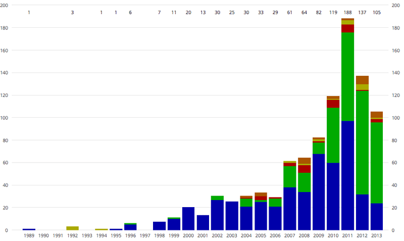
A quiet milestone in modern astronomy may soon come to pass.  As of today, The Extrasolar Planets Encyclopedia lists a current tally of 998 extrasolar planets across 759 planetary systems. And although various tabulations differ slightly, very soon we should be living in an era where over one thousand exoplanets are known.

The history of exoplanet discovery has paralleled the course of the modern age of astronomy. It’s strange to think that a generation has already grown up over the past two decades in a world where knowledge of extrasolar planets is a given. I remember hearing of the promise of such detections growing up in the 1970’s, as astronomers put the odds at detection of planets beyond our solar system in our lifetime at around 50%.

A "Periodic Table of Exoplanets" Credit: PHL @ UPR Arecibo.
A “Periodic Table of Exoplanets” Credit: PHL @ UPR Arecibo.

Sure, there were plenty of false positives long before the first true discovery was made. 70 Ophiuchi was the site of many claims, starting with that of W.S. Jacob of the Madras Observatory way back in 1855. The high proper motion exhibited by Barnard’s Star at six light years distant was also highly scrutinized throughout the 20th century for claims of an unseen companion causing it to wobble. Ironically, Barnard’s Star still hasn’t made it into the pantheon of stars boasting planetary worlds.

A portrait of the HR8799 planetary system as imaged by the Hale Telescope. (Credit: NASA/JPL-Caltech/Palomar Observatory).

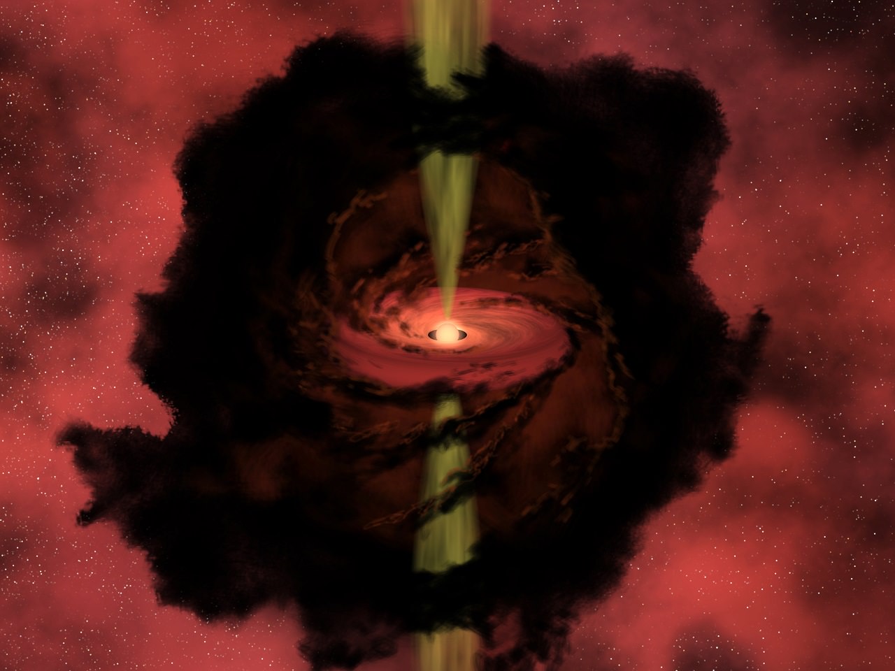
But the first verified claim of an exoplanetary system came from a bizarre and unexpected source: a pulsar known as PSR B1257+12, which was discovered to host two worlds in 1992. This was followed by the first discovery of a world orbiting a main sequence star, 51 Pegasi in 1994. I still remember getting my hands on the latest issue of Astronomy magazine— we got our news, often months later, from actual paper magazines in those days —announcing “Planet Discovered!” on the cover.

Most methods and techniques used to discover exoplanets rely on either radial velocity or dips in the light output of a star from a transiting world. Both have their utility and drawbacks. Radial velocity looks for shifts in the star’s spectra as an unseen companion tugs it around a common center of mass. Though effective, it can only place a lower limit on the planet’s mass… and it’s biased towards worlds in short orbits. This is one reason that “hot Jupiters” have dominated the early exoplanet catalog: we hadn’t been looking for all that long.

Another method famously employed by surveys such as the Kepler space telescope is the transit detection method. This allows a much more refined estimate of a planet’s mass and orbit, assuming it transits the disk of its host star as seen from our Earthly vantage point in the first place, which most don’t.

A size comparision of exoplanets versus composition. (Credit: Marc Kuchner/NASA/GSFC).

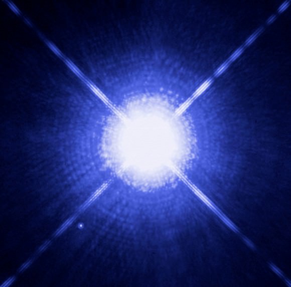
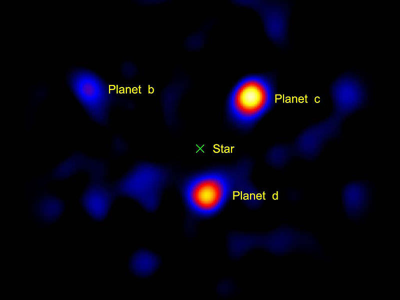
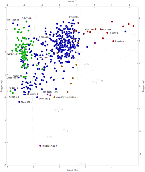
Direct detection via occulting the host star is also coming of age. One of the first exoplanets directly imaged was Fomalhaut b, which can be seen changing positions in its orbit from 2004 to 2006.

Gravitational microlensing has also bared planetary fruit, with surveys such as MOA (Microlensing Observations in Astrophysics) and OGLE (the Optical Gravitational Lensing Experiment) catching brief lensing events as an unseen body passes in front of a background star. Distant free-ranging rogue planets can only be detected via this method.

More exotic techniques also exist, such as relativistic beaming (sounding like something out of Star Trek). Other methods include searches for tiny light variations as an illuminated planet orbits its host star, deformities caused by ellipsoidal variations as massive planets orbit a star, and infrared detections of circumstellar disks. We’re always amazed at the wealth of data that can be teased out of a few dim photons of light.

A scatter plot of exoplanet discoveries as of 2010 mass versus semi-major axis. Select exoplanets are labeled. A majority were detected via radial velocity (blue) and the transiting method (green). The remainder were detected by other methods (click here for a full discription). Graph in the Public Domain.
A scatter plot of exoplanet discoveries as of 2010 displaying mass versus semi-major axis. Select exoplanets are labeled. A majority were detected via radial velocity (blue) and the transiting method (green). The remainder were detected by other methods (click here for a full description). Graph in the Public Domain.

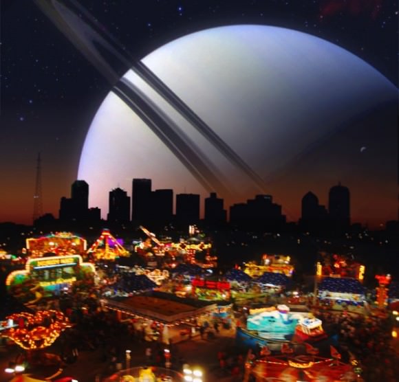
Universe Today has grown up with exoplanet science, from reporting on the hottest, fastest, and other notable “firsts”. A bizarre menagerie of worlds are now known, many of which defy the imagination of science fiction writers of yore. Want a world made of diamond, or one where it rains glass? There’s now an “exoplanet for that”.

Exoplanet news has almost gone from the incredible to the routine, as Tatooine-like worlds orbiting binary stars and systems with worlds in bizarre resonances are announced with increasing frequency.

Exoplanet surveys also have a capacity to peg down that key fp factor in the famous Drake equation, which asks us “what fraction of stars have planets”. It’s been long suspected that stars with planets are the rule rather than the exception, and we’re just now getting hard data to back that assertion up.

Missions, such as NASA’s Kepler space telescope and CNES/ESA CoRoT space telescope have swollen the ranks of extrasolar worlds. Kepler recently ended its career staring off in the direction of the constellations Cygnus, Hercules and Lyra and still has over 3,200 detections awaiting confirmation.

Exoplanet discoveries by year as of October 2013, color coded by method. Blue=radial velocity, Green=transiting, Yellow=timing, Red=direct imaging, Orange=microlensing

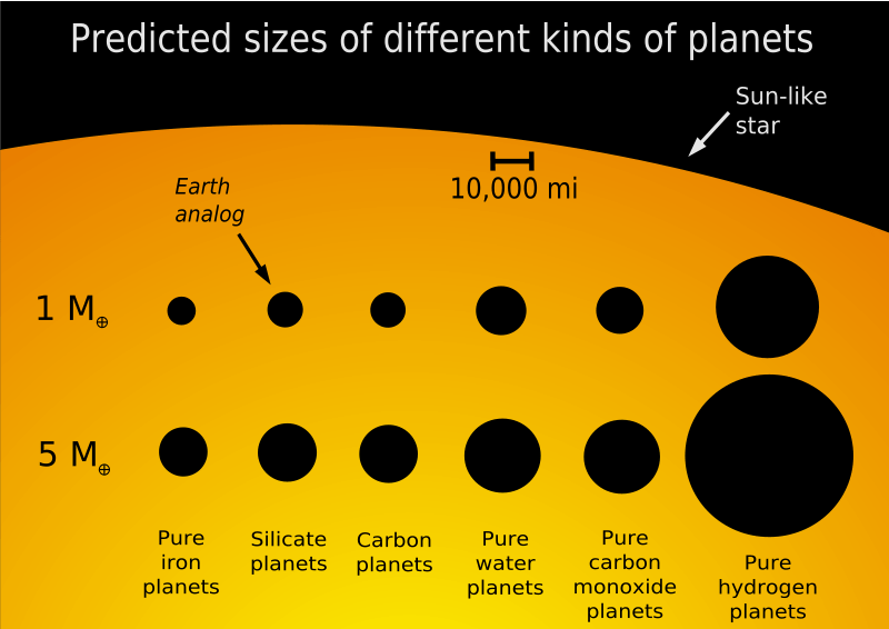
But is a given world Earthlike, or just Earth-sized? That’s the Holy Grail of modern exoplanet detection: an Earth-sized world orbiting in a star’s habitable zone. We’re cautious every time the latest “Earth-twin” makes its way into the headlines. From the perspective of an intergalactic astronomer, Venus in our own solar system might appear to fit the bill, though I wouldn’t bank the construction of an interstellar ark on it and head there just yet.

Exoplanet science has definitely come of age, allowing us to finally begin characterization of solar systems and give us some insight into solar system formation.

But perhaps what will be the most enduring legacy is what the discovery of extrasolar planets tells us about ourselves. How common (or rare) is the Earth? How typical is the story of our solar system? If the “first 1,000” are any indication, we strongly suspect that terrestrial planets come in enough distinct varieties or ”flavors” to make Baskin Robbins envious.

And the future of exoplanet science looks bright indeed. One proposed mission, known as the Fast INfrared Exoplanet Spectroscopy Survey Explorer, or FINESSE, would target exoplanet atmospheres, if given the go ahead for a 2017 launch. Another proposal, known as the Wide Field Infrared Survey Telescope, or WFIRST, would search for microlensing events starting in 2023. A mission that scientists would love to fly that always seems to be shelved is known as the Terrestrial Planet Finder.

But the exoplanet hunting mission that’s closest to launch is the Transiting Exoplanet Survey Satellite, or TESS. Unlike Kepler, which stares at a single patch of sky, TESS will be an all-sky survey looking at a half million stars.

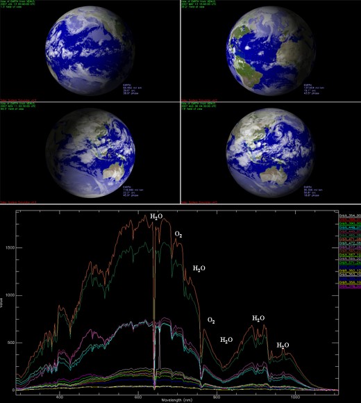
We’re also just approaching an era where spectroscopy may allow us to detect exomoons and the chemistry taking place on these far off exoworlds. An example of an exciting discovery would be the detection of a chemical such as chlorophyll, a chemical that we know on Earth only exists as the result of life. But what a tantalizing discovery a blip on a graph would be, when what we humans really want to see is the vista of those far-flung alien forests!

Such is the exciting era we live in. Congratulations, humanity, on detecting 1,000 exoplanets… here’s to a thousand more!

Wet Asteroid’s Remains Found In Old Star That Could Have Hosted Habitable Planets

Artist's impression of a rocky and water-rich asteroid being torn apart by the strong gravity of the white dwarf star GD 61. Credit: Mark A. Garlick, space-art.co.uk, University of Warwick and University of Cambridge

Remains of a water-filled asteroid are circling a dying white dwarf star, right now, about 150 light-years from us. The new find is the first demonstration of water and a rocky surface in a spot beyond the solar system, researchers say.

The discovery is exciting to the astronomical team because, according to them, it’s likely that water on Earth came from asteroids, comets and other small bodies in the solar system. Finding a watery rocky body demonstrates that this theory has legs, they said. (There are, however, multiple explanations for water on Earth.)

“The finding of water in a large asteroid means the building blocks of habitable planets existed – and maybe still exist – in the GD 61 system, and likely also around substantial number of similar parent stars,” stated lead author Jay Farihi, from Cambridge’s Institute of Astronomy.

Earth’s oxygen and water as detected by Venus Express (ESA)

“These water-rich building blocks, and the terrestrial planets they build, may in fact be common – a system cannot create things as big as asteroids and avoid building planets, and GD 61 had the ingredients to deliver lots of water to their surfaces. Our results demonstrate that there was definitely potential for habitable planets in this exoplanetary system.”

More intriguing, however, is researchers found this evidence in a star system that is near the end of its life. So the team is framing this as a “look into our future”, when the Sun evolves into a white dwarf .

The water likely came from a “minor planet” that was at least 56 miles (90 kilometers) in diameter. Its debris was pulled into the atmosphere of the star, which was then examined by spectroscopy. This study revealed the ingredients of rocks inside the star, including magnesium, silicon and iron. Researchers then compared these elements to how abundant oxygen was, and found that there was in fact more oxygen than expected.

White Dwarf Star
White Dwarf Star

“This oxygen excess can be carried by either water or carbon, and in this star there is virtually no carbon – indicating there must have been substantial water,” stated co-author Boris Gänsicke, from the University of Warwick.

“This also rules out comets, which are rich in both water and carbon compounds, so we knew we were looking at a rocky asteroid with substantial water content – perhaps in the form of subsurface ice – like the asteroids we know in our solar system such as Ceres.”

The measurements were obtained in ultraviolet with the Hubble Space Telescope’s cosmic origins spectrograph. What’s more, the researchers suspect there are giant exoplanets in the area because it would take a huge push to move this object from the asteroid belt — a push that most likely came from big planet.

“This supports the idea that the star originally had a full complement of terrestrial planets, and probably gas giant planets, orbiting it – a complex system similar to our own,” Farihi added.

The discovery was recently published in Science.

Source: University of Cambridge

Masked Starbirth Mapped In New Milky Way Survey

Artist's conception of a star being born, within a protective shroud of gas and dust. New research shows that magnetic winds aid the growth of both protostars and SMBHs. Credit: NASA

Stars are born in private. Hidden in dust and gas clouds, these bright beacons in the universe slowly coalesce. All that debris makes it hard to spot the stars, but mapping out the pockets of starbirth is a good start to understanding what is going on inside.

A new survey tracked down 6,000 of these areas in our galaxy (the Milky Way), with the aim of understanding more about what happens when stars are just starting to come together. Most surveys, the team says, focus more on the “protostar” stage, when these objects are starting to look recognizably like stars.

“Starless clumps have only been detected in small numbers to date,” stated Yancy Shirley, an astronomer with the University of Arizona’s Steward Observatory who led the research. “Now, for the first time, we have seen this earliest phase of star formation, before a cluster actually forms, in large numbers in an unbiased way.”

Artist's conception of the Milky Way galaxy. Credit: Nick Risinger
Artist’s conception of the Milky Way galaxy. Credit: Nick Risinger

These areas are difficult to peer through in visible light, but radio works just fine. The astronomers used the Sub-Millimeter Telescope at the Arizona Radio Observatory to conduct the survey, which looks at “all parts of the galactic plane visible from the northern hemisphere”, the team says.

It’s the first survey to show the environments where different stages of starbirth take place. While the team did not immediately disclose their plans for a follow-up in a press release, they state that one aim of mapping these areas is to “better understand how the properties of these regions change as star formation progresses.”

Read all about the survey in The Astrophysical Journal, or the preprint version on Arxiv.

Source: University of Arizona

Future Supernova Is Surrounded By Hydrogen Clouds

A "super star cluster", Westerlund 1, which is about 16,000 light-years from Earth. It can be found in the southern constellation of Ara. The picture was taken from the European Southern Observatory's VLT Survey Telescope. Credit: ESO/VPHAS+ Survey/N. Wright

The faint green glow you see in that picture is not an early harbringer of Hallowe’en spooks. It’s hydrogen gas clouds found recently nearby W26, a future supernova in the star cluster Westerlund 1.

The European Southern Observatory’s VLT Survey Telescope in Chile spotted the hydrogen in the cluster, which has hundreds of huge stars that are only believed to be a few million years old. (Our solar system, by comparison, is about 4.5 billion years old.)

“Such glowing clouds around massive stars are very rare, and are even rarer around a red supergiant— this is the first ionised nebula discovered around such a star,” the European Southern Observatory stated.

“W26 itself would be too cool to make the gas glow; the astronomers speculate that the source of the ionizing radiation may be either hot blue stars elsewhere in the cluster, or possibly a fainter, but much hotter, companion star to W26.”

Funny enough, the nebula that surrounds the red supergiant is similar to the one surrounding SN1987A, a star that exploded as a fairly bright supernova in 1987. “Studying objects like this new nebula around W26 will help astronomers to understand the mass loss processes around these massive stars, which eventually lead to their explosive demise,” ESO added.

Source: European Southern Observatory

Carnival of Space #323

Carnival of Space. Image by Jason Major.

This week’s Carnival of Space is hosted by Allen Versfeld at his Urban Astronomer blog.

Click here to read Carnival of Space #323.

And if you’re interested in looking back, here’s an archive to all the past Carnivals of Space. If you’ve got a space-related blog, you should really join the carnival. Just email an entry to [email protected], and the next host will link to it. It will help get awareness out there about your writing, help you meet others in the space community – and community is what blogging is all about. And if you really want to help out, sign up to be a host. Send an email to the above address.

This Week’s Penumbral Lunar Eclipse and the Astronomy of Columbus

(Photo by Author)

You can always count on an eclipse to get you out of a delicate situation. Today is Columbus Day in the United States and Thanksgiving north of the border in Canada. Later this week also marks the start of the second eclipse season for 2013. Today, we thought we’d take a look at the circumstances for the first eclipse of the season kicking off this coming Friday night, October 18, as well as the fascinating role that eclipses played in the life and times of Christopher Columbus.

Friday’s event is a penumbral lunar eclipse, meaning that the Full Moon will only pass through the outer bright rim of the Earth’s shadow. Such events are subtle affairs, as opposed to total and partial lunar eclipses, which occur when the Moon enters the dark inner core, or umbra, of the Earth’s shadow. Still, you may just be able to notice a slight dusky shading on the lower southern limb of the Moon as it flirts with the umbra, barely missing it around the time of central eclipse at 23:51 Universal Time/ 7:51 PM Eastern Daylight Saving Time. Friday night’s penumbral is 3 hours and 59 minutes in duration, and 76.5% of the disk of the Moon will be immersed in the penumbra at maximum eclipse.

eclipse
The visibility footprint and circumstances of this week’s penumbral lunar eclipse. (Credit: Fred Espenak/NASA/GSFC).

Key Events occurring on Friday, October 18th:

21:50UT/5:50PM EDT: 1st contact with the Earth’s shadow.

23:51UT/7:51PM EDT: Mid-eclipse.

01:49UT(Oct 19th)/9:49PM EDT: Last contact. Eclipse ends.

The eclipse will be underway at moonrise for North and South America and occur at moonset for central Asia— Africa and Europe will see the entire eclipse. Standing on Earth’s Moon, an observer on the nearside would see a partial solar eclipse.

A simulation of Friday's lunar eclipse, looking back from Earth Moon at mid-eclipse. (Credit:
A simulation of Friday’s lunar eclipse, looking back from Moon at mid-eclipse. (Wikimedia Commons graphic in the Public Domain).

This eclipse is the 3rd and final lunar eclipse of 2013, and the 5th overall. It’s also the first in a series of four descending node eclipses, including the total lunar eclipse of October 8th next year.   It’s also the 52nd eclipse of 72 in the lunar saros series 117, which started on April 3rd, 1094 and will end with a final lunar eclipse on May 15th, 2356. Saros 117 produced its last total lunar eclipse in 1815 and its final partial in 1941.

Though penumbrals are slight events, we’ve been able to notice an appreciable difference before, during and after the eclipse photographically:

Penumbral I
Can you spy the difference? The May 18th, 2002 penumbral lunar eclipse before (left) and during mid-eclipse (right). Photos by Author.

Be sure to use identical exposure settings to catch this effect. Locations where the Moon rides high in the sky also stand the best chance of imaging the faint penumbral shading, as the Moon will be above the discoloring effects of the thicker air mass low to the horizon.

The Moon reaches descending node along the ecliptic about 20 hours after the end of the eclipse, and reaches apogee just over six days later on October 25th. The October Full Moon is also known as the Hunter’s Moon, providing a bit of extra illumination on the Fall hunt.

And this sets us up for the second eclipse of the season the next time the Moon crosses an ecliptic node, a hybrid (annular-total) solar eclipse spanning the Atlantic and Africa on November 3rd. More to come on that big ticket event soon!

In Columbus’s day, the Moon was often used to get a rough fix of a ship’s longitude at sea. Columbus was especially intrigued with the idea of using lunar eclipses to determine longitude. If you can note the position of the Moon in the sky from one location versus a known longitude during an event— such as first contact of the Moon with the Earth’s umbra during an eclipse —you can gauge your relative longitude east or west of the point. The sky moves 15 degrees, or one hour of right ascension overhead as we rotate under it. One of the earliest records of this method comes to us from Ptolemy, who deduced Alexander the Great’s position 30 degrees (2 hours) east of Carthage during the lunar eclipse of September 20th, 331 B.C. Alexander noted that the eclipse began two hours after sunset from his locale, while in Carthage it was recorded that the eclipse began at sunset.

A Jacob's crossstaff, a simple tool for measuring angles in the sky. (Photo by Author).
A Jacob’s cross staff, a simple tool for measuring angles in the sky. (Charles Towne Landing Historic Site Museum, Photo by Author).

Columbus was a student of Ptolemy, and used this method during voyages to and from the New World during the lunar eclipses of September 14th, 1494 and February 29, 1504. Of course, such a method is only approximate. The umbra of the Earth often appears ragged and indistinct on the edge of the lunar disk at the start of an eclipse, making it tough to judge the actual beginning of an eclipse by more than ten of minutes or so. And remember, you’re often watching from the pitching deck of a ship to boot!

Another problem also plagued Columbus’s navigation efforts: he favored a smaller Earth than we now know is reality. Had he listened to another Greek astronomer by the name of Eratosthenes, he would’ve gotten his measurements pretty darned close.

An eclipse also saved Columbus’s butt on one occasion. The story goes that tensions had come to a head between the locals and Columbus’s crew while stranded on the island of Jamaica in 1504. Noting that a lunar eclipse was about to occur on March 1st  (the evening of February 29th for North America), Columbus told the local leader that the Moon would rise “inflamed with wrath,” as indeed it did that night, right on schedule. Columbus then made a great show of pretending to pray for heavenly intersession, after which the Moon returned to its rightful color.  This kept a conniving Columbus and his crew stocked in supplies until a rescue ship arrived in June of that year.

A depiction of the 1504 lunar eclipse from the 1879 text Astronomie Populare by Camille Flammarion.
A depiction of the 1504 lunar eclipse from the 1879 text Astronomie Populare by Camille Flammarion.

Be sure to check out this Friday’s penumbral eclipse, and amaze your friends with the prediction of the next total lunar eclipse which occurs on U.S. Tax Day next year on April 15th, 2014. Can you do a better job of predicting your longitude than Columbus?

Astronomers Stress the Need for Characterizing the Population of Nearby Potential Earth-Impactors

Frame grab from a video of the Feb. 15, 2013 Russian fireball by Aleksandr Ivanov

The meteor explosion over Russia in February 2013 raised concerns that even small asteroid impactors may wreak some havoc given our heavily populated cities.  A new study by NASA scientists aims to improve our understanding of such asteroids that are lurking in Earth’s vicinity.  The team, led by Amy Mainzer, noted that only a mere fraction of asteroids comparable in size to the object that exploded over Russia have been discovered, and their physical properties are poorly characterized.

The team derived fundamental properties for over a hundred near-Earth objects, and determined that many are smaller than 100 meters.  Indeed, the team notes that, “In general … [asteroids] smaller than 100-m are only detected when they are quite close … and the smallest … were detected when they were only 2-3 lunar distances away from Earth.”  

Essentially, a large fraction of these bodies may go undetected until they strike Earth, analogous to the case of the asteroid that exploded over Russia in February.

The team’s results rely partly on observations from the Wide-field Infrared Survey Explorer (WISE), which is a space-based telescope that mapped the entire sky in the mid-infrared. Observations taken in the infrared, in concert with those taken in the optical, can be used to infer the fundamental properties of asteroids (e.g., their diameter and chemical composition).

On a somewhat positive note, Mainzer remarks that 90% of near-Earth asteroids larger than 1-km are known, and those potential impactors are most worrisome as they may cause widespread fatalities.  The dinosaurs suffered a mass-extinction owing, at least in large part, to a 10-km impactor that struck Earth 65 million years ago.   However, Mainzer notes that the survey completeness drops to 25% for nearby 100-m asteroids, and it is likely to be less than 1% for 20-m asteroids like that which exploded over Russia (Chelyabinsk).  The Tunguska event (see the image below) is likewise speculated to have been on the order of that latter size.

In 1908 the Tunguska impactor toppled millions of trees in a rather remote part of Siberia.  The new study by Mainzer and coauthors aimed to better characterize the population of Tunguska-sized asteroids lurking in the vicinity of the Earth.
In 1908 the Tunguska meteor explosion toppled millions of trees in a rather remote part of Siberia. A new study by Mainzer et al. 2013 characterized 100+ objects lurking in the vicinity of the Earth that are on the order of the Tunguska impactor.

The team highlights that approximately 10,000 near-Earth objects have been discovered to date, 900 of which are 1-km or larger, and 3500 objects appear to be 100-m or smaller.  “Because their small sizes usually make them undetectable until they are very nearby the Earth, it is often difficult for the current suite of asteroid surveys and follow-up telescopes to track them for very long.

Consequently, the fraction of the total population at small sizes that has been discovered to date remains very low,” noted Mainzer.

In closing, Mainzer emphasizes that, “It is, however, clear that much work remains to be done to discover and characterize the population of very small NEOs [near-Earth objects].”


The Mainzer et al. 2013 findings have been accepted for publication in the Astrophysical Journal (ApJ), and a preprint is available on arXiv.  Coauthors on the study are J. Bauer, T. Grav, J. Masiero, R. M. Cutri, E. L. Wright, C. R. Nugent, R. Stevenson, E. Clyne, G. Cukrov, and F. Masci.

Technicolor Auroras? A Reality Check

Beautiful red and green aurora the night of Oct. 1-2, 2013. See below for how it appeared to the eye. Details: 20mm lens, f/2.8, ISO 1600 and 25-second exposure. Credit: Bob King

I shoot a lot of pictures of the northern lights. Just like the next photographer, I thrill to the striking colors that glow from the back of my digital camera. When preparing those images for publication, many of us lighten or brighten the images so the colors and forms stand out better. Nothing wrong with that, except most times the aurora never looked that way to our eyes.

Shocked? I took the photo above and using Photoshop adjusted color and brightness to match the naked eye view. Credit: Bob King
Surprised? I took the photo above and using Photoshop adjusted color and brightness to match the naked eye view. Notice the green tinge in the bright arc at bottom. The rays were colorless. Credit: Bob King


The colors you see in aurora photos ARE real but exaggerated because the pictures are time exposures. Once the camera’s shutter opens, light accumulates on the electronic sensor, making faint and pale subjects bright and vivid. The camera can’t help it, and who would deny a photographer the chance to share the beauty? Most of us understand the magic of time exposures and factor in a mental fudge factor when looking at astronomical photos including those of the aurora.

But photos can be misleading, especially so for beginners, who might anticipate “the second coming” when they step out to watch the northern lights only to feel disappointment at the real thing. Which is too bad, because the real aurora can make your jaw drop.

A massive wall of bright purple and green rays from July 20, 2012. Details: 16mm at f/2.8, ISO 800 and 20 second exposure. Credit: Bob King

That’s why I thought it would instructive to take a few aurora photos and tone them down to what the eye normally sees.  Truth in advertising you know. I’ve also started to include disclaimers in my captions when the images show striking crimson rays. Veteran aurora watchers know that some of the most memorable auroral displays glow blood-red, but most of the ruddy hues recorded by the camera are simply invisible to the eye. Our eyes evolved their greatest sensitivity to green light, the slice of the rainbow spectrum in which the sun shines most intensely. We’re slightly less sensitive to yellow and only a 1/10 as sensitive to red.

Image adjusted to better represent the visual view. Credit: Bob King
Image adjusted to better represent the visual view. Most auroras are between 60 and 150 miles high, but occasionally reach to 400 miles. Credit: Bob King

A typical aurora begins life as a pale white band low in the northern sky. If we’re lucky, the band intensifies, crosses the color threshold and glows pale green. Deeper and brighter greens are also common in active and bright auroras, but red is elusive because are eyes are far less sensitive to it than green. Often a curtain of green rays will be topped off by red, blue or purple emission recorded with sumptuous fidelity in the camera. What does the eye see? Smoky, colorless haze with hints of pink. Maybe.

Again, this doesn’t mean we only see green and white. I’ve watched brilliant (pale) green rays stretch from horizon to zenith with their bottoms bathed in rosy-purple, a most wonderful sight. Another factor to keep in mind is dark adaption – the longer you’ve been out under a dark sky, the more sensitive your eyes will be to whatever color might be present. At night, however, we’re mostly color blind, relying on our low-light-sensitive rod cells to get around. Cone cells, fine-tuned for color vision, are activated only when light intensity reaches certain thresholds. That happens often when it comes to auroral green but less so with other colors to which our cells are less responsive.

Excitation of oxygen and nitrogen atoms and molecules by incoming solar electrons causes them to give off specific colors shown here. Credit: NCAR
Incoming auroral electrons excite oxygen and nitrogen atoms and molecules which then shoot out photons of light at specific wavelengths when they return to their ground states. Oxygen beams light at 557.7 (green) and 603 (red) nanometers. Credit: NCAR

Auroral colors originate when electrons from the sun spiral down Earth’s magnetic field lines like firemen on a firepole and slam into oxygen and nitrogen atoms in Earth’s upper atmosphere between 60 and 150 miles (96-240 km) high. Here’s a breakdown of color, atom and altitude:

* Green – oxygen atoms 60-93 miles up (100-150 km)
* Red – oxygen atoms from 93-155 miles (150-250 km)
* Purple – molecular nitrogen up to 60 miles (100 km)
* Blue/purple – molecular nitrogen ions above 100 miles (160 km)

When an electron strikes an oxygen atom for instance, it bumps one of the oxygen’s electrons to a higher energy level. When that electron drops back down to its previous rest or ground state, it emits a photon of green light. Billions of atoms and molecules, each cranking out tiny flashes of light, make an aurora. It takes about 3/4 second for that electron to drop and the atom to release a photon before it’s given another kick from a solar electron. Most auroras are rich with oxygen emission.

The layers of our atmosphere showing the altitude of the most common auroras. Credit: Wikimedia Commons

Higher up, where the air’s so thin it’s identical to a hard vacuum, collisions between atoms happen only about every 7 seconds. With lots of time on their hands, oxygen electrons can transition down to their lowest energy level inside the atom, releasing a photon of red light instead of green. That’s why tall rays often show red tops especially in time exposure photos.

Only during very active geomagnetic storms, when electrons penetrate to low levels in the atmosphere, are they able to excite molecules of nitrogen, giving rise to the familiar purple fringes at the bottoms of bright rays. Bombarded molecular nitrogen ions at high altitude release a deep blue-purple light. Rarely visible to the eye, I did record it one night in the camera.

A striking coronal aurora in Feb. 1999 photographed on film. The red in this aurora was obvious to the naked eye but appeared more like the Photoshopped version at right. Credit: Bob King

While videos hint at how wildly dynamic auroras can be, they’re no substitute for seeing one yourself. That’s why I never seem to get to bed when that first tempting glow appears over the northern horizon. Colorful or colorless, you’ll be astonished at how the aurora constantly re-invents itself in a multitude of forms from arcs to rays to flaming patches and writhing curlicues. Don’t miss the chance to see one. If there’s one thing that looks absolutely unearthly on this green Earth, it’s the aurora borealis. Click HERE for a guide on when and where to watch for them.


Where Did the Earth’s Water Come From?

Where Did the Earth's Water Come From?

This question comes from Andrew Bumford and Steven Stormont.

In a previous episode I’ve talked about how the entire Solar System collapsed down from a cloud of hydrogen and helium left over from the Big Bang. And yet, we stand here on planet Earth, with all its water. So, how did that H20 get to our planet? The hydrogen came from the solar nebula, but where did the oxygen come from?
Here’s the amazing part.

The oxygen came from stars that lived and died before our Sun was even born. When those stars puffed out their final breaths of oxygen, carbon and other “metals”, they seeded new nebulae with the raw material for new worlds. We owe our very existence to the dead stars that came before.

When our Sun dies, it’ll give up some of its heavier elements to the next generation of stars. So, mix hydrogen together with this donated oxygen, and you’ll get H20. It doesn’t take any special process or encouragement, when those two elements come together, water is the result.

But how did it get from being spread across the early Solar System to concentrating here on Earth, and filling up our oceans, lakes and rivers? The exact mechanism is a mystery. Astronomers don’t know for sure, but there are a few theories:

Idea #1: impacts. Take a look at the craters on the Moon and you’ll see that the Solar System was a busy place, long ago. Approximately 3.8 to 4.1 billion years ago was the Late Heavy Bombardment period, when the entire inner Solar System was pummeled by asteroids. The surfaces of the planets and their moons were heated to molten slag because of the non-stop impacts. These impactors could have been comets or asteroids.

Comets are 80% water, and would deliver vast amounts of water to Earth, but they’re also volatile, and would have a difficult time surviving the harsh radiation of the young Sun. Asteroids have a lower ratio of water, but they could protect that water a little better, delivering less with each catastrophic impact.

A false-color, visible-light image of Comet ISON taken with Hubble's Wide Field Camera 3. Credit: NASA, ESA, and the Hubble Heritage Team (STScI/AURA)
A false-color, visible-light image of Comet ISON taken with Hubble’s Wide Field Camera 3. Credit: NASA, ESA, and the Hubble Heritage Team (STScI/AURA)

Astronomers have also found many hybrid objects which contain large amounts of both rock and water. It’s hard to classify them either way.

Idea #2 is that large amounts of water just came directly from the solar nebula. As we orbited around the young Sun, it passed through the water-rich material in the nebula and scooped it up. Gravitational interactions between the planets would have transferred material around the Solar System, and it would have added to the Earth’s volume of water over hundreds of millions of years.

Of course, it’s entirely possible that the answer is “all of the above”. Asteroids and comets and the early solar nebula all delivered water to the Earth. Where did the Earth’s water come from? Astronomers don’t know for sure. But I’m sure glad the water is here; life here wouldn’t exist without it.

Tranquil Galaxy With Petals Shows Clues To A Violent Past

PGC 6240, a petal-like galaxy that probably was altered by a galactic merger. Credit: ESA/Hubble & NASA with acknowledgement to Judy Schmidt

Across the universe, some 350 million light-years away, lies a galaxy that looks like it has white rose petals. Don’t let the tranquil appearance of PGC 6240 fool you as to its past, however. This galaxy in Hydrus (The Water Snake) likely was dramatically altered by a galactic merger.

There’s a bunch of evidence pointing to this. There are “star shells” of globular clusters around the galaxy, but they’re distributed unevenly — some are close in, some are way out in the distant suburbs. Also, “several wisps of material have been thrown so far that they appear to be almost detached from the galaxy altogether,” stated the Hubble European Space Agency Information Centre.

“The most likely explanation for both the galaxy’s stacked shell structure and the unexpectedly young star clusters is that PGC 6240 merged with another galaxy at some point in the recent past,” the agency added.

“Such a merger would send ripples through the galaxy and disrupt its structure, forming the concentric shells of material seen here. It would also ignite a strong burst of star formation in the galaxy, which would then trigger similar activity in nearby space — leading to the creation of new, younger globular clusters around PGC 6240.”

Source: The Hubble European Space Agency Information Centre