Earth Observation Archives

June 10, 2011April 26, 2016 by Nancy Atkinson

Aquarius Satellite Launches to Observe Earth’s Oceans

A picture-perfect launch on a Delta II rocket from Vandeberg Air Force Base in California sent the newest satellite into orbit. The Aquarius/SAC-D spacecraft lifted off June 10, 2011 at 7:20 a.m. PDT (1420 UTC) to gather global measurements of ocean surface salinity, leading to a better understanding of ocean circulation, climate and Earth’s water cycle. NASA’s Aquarius instrument is part of the SAC-D spacecraft built by CONAE, Argentina’s space agency.

Continue reading “Aquarius Satellite Launches to Observe Earth’s Oceans”

May 24, 2011January 18, 2016 by Nancy Atkinson

Joplin, Missouri Tornado Seen From Space

This video from NOAA’s GOES geostationary satellite shows the development of the supercell storm that produced the devastating tornado that struck Joplin, Missouri. Here you can see the storm develop over Missouri, Oklahoma, Kansas state lines on May 22, 2011 between 12:44pm to 7:15pm CDT. This was part of the great wave of severe storms that swept across the central United States, with tornado warnings from Minneapolis to Dallas. The most damaging storm struck Joplin at 5:30 pm local time (2230 UTC), killing at least 116 people.

Below is imagery from the Tropical Rainfall Measuring Mission satellite (TRMM).
Continue reading “Joplin, Missouri Tornado Seen From Space”

May 24, 2011December 24, 2015 by VirtualAstro

Coming Soon – Night Shining Noctilucent Clouds

Noctilucent Cloud Display Credit: Adrian West

[/caption]

Soon you may see an eerie spectacle on clear summer nights if you are located at latitudes between 50° and 70° north and south of the equator: Noctilucent Clouds.

These ghostly apparitions are a delight to see and are quite rare. It is incredibly difficult to predict exactly when they will appear, but we do know they should begin to appear soon.

The season for Noctilucent Clouds (Noctilucent = Latin for “Night Shining”) starts early June and continues into late July. They are seen just after dusk, or before dawn and an apparition can last around an hour.

These mysterious clouds, with their bizarre tenuous wispy shapes reminiscent of ripples in sand or the changing surface of a pool of water, spread like a glowing web across the northern sky. Colours can range from brilliant whites, with tinges of blue, pink and orange.

Formed by tiny ice crystals, they are the highest clouds in the Earth’s atmosphere, located in the mesosphere at altitudes of around 76 to 85 kilometers (47 to 53 miles) almost at the edge of space.

They are normally too faint to be seen, and are visible only when illuminated by sunlight from below the horizon, while the lower layers of the atmosphere are in the Earth’s shadow. Noctilucent clouds are not fully understood and are a recently discovered meteorological phenomenon, only being recorded for about 120 years.

Noctilucent clouds can only form under very restrictive conditions, and their occurrence can be used as a guide to changes in the upper atmosphere. Since their relatively recent classification, the occurrence of noctilucent clouds appears to be increasing in frequency, brightness and extent.

There is evidence that the relatively recent appearance of noctilucent clouds and their gradual increase, may be linked to climate change. Another recent theory is that some of these bright displays come from particulates and water vapour in the atmosphere left over from Space Shuttle launches.

How can you see them? Over the next couple of months look north during dusk and dawn and try and spot this mysterious and elusive phenomenon. They are best seen when the sun is between 6 and 16 degrees below the horizon, and seem to occur more frequently in the Northern hemisphere than the Southern.

Good luck!

Noctilucent clouds over Blair, Nebraska, USA. Credit: Mike Hollingshead

May 23, 2011January 18, 2016 by Nancy Atkinson

The View from 100,000 Feet

I love these student projects that send a camera via a balloon high in the atmosphere to film the view of Earth below. Here’s another from a group of German students who were able to film in HD from an altitude of more than 100,000 ft. (30,480 meters). Enjoy the music, too.

“Our challenge was to survive ambient air pressures as low as 1/100th of an atmosphere, temperatures as low as -60°C and finally to locate and recover the Camera,” Tobias Lohf wrote UT. “We had a HD-Cam, GPS tracker and a heating pad on board, and all the construction had a total weight of about 1kg.”

The rest of the team included Marcel Dierig, Tobias Stodieck, Tristan Eggers and Marvin Rissiek and they hope to inspire other students to try the same project. “All you need need is a camera, weather balloon and Duct Tape,” they said.

May 17, 2011December 24, 2015 by Nancy Atkinson

New Satellite Will ‘Taste’ Earth’s Salty Seas from Orbit

Artist's concept of the Aquarius/SAC-D spacecraft, a collaboration between NASA and Argentina's space agency, with participation from Brazil, Canada, France and Italy. Aquarius, the NASA-built primary instrument on the spacecraft, will take NASA's first space-based measurements of ocean surface salinity, a key missing variable in satellite observations of Earth that links ocean circulation, the global balance of freshwater and climate. The mission is scheduled to launch in June. Image credit: NASA

[/caption]

From a JPL press release:

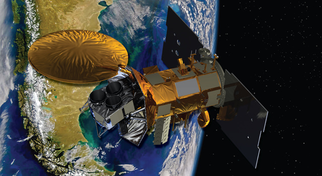
Final preparations are under way for the June 9 launch of the international Aquarius/SAC-D observatory. The mission’s primary instrument, Aquarius, will study interactions between ocean circulation, the water cycle and climate by measuring ocean surface salinity.

Engineers at Vandenberg Air Force Base in California are performing final tests before mating Aquarius/SAC-D to its Delta II rocket. The mission is a collaboration between NASA and Argentina’s space agency, Comision Nacional de Actividades Espaciales (CONAE), with participation from Brazil, Canada, France and Italy. SAC stands for Satelite de Applicaciones Cientificas. Aquarius was built by NASA’s Jet Propulsion Laboratory in Pasadena, Calif., and the agency’s Goddard Space Flight Center in Greenbelt, Md.

In addition to Aquarius, the observatory carries seven other instruments that will collect environmental data for a wide range of applications, including studies of natural hazards, air quality, land processes and epidemiology.

The mission will make NASA’s first space observations of the concentration of dissolved salt at the ocean surface. Aquarius’ observations will reveal how salinity variations influence ocean circulation, trace the path of freshwater around our planet, and help drive Earth’s climate. The ocean surface constantly exchanges water and heat with Earth’s atmosphere. Approximately 80 percent of the global water cycle that moves freshwater from the ocean to the atmosphere to the land and back to the ocean happens over the ocean.

Salinity plays a key role in these exchanges. By tracking changes in ocean surface salinity, Aquarius will monitor variations in the water cycle caused by evaporation and precipitation over the ocean, river runoff, and the freezing and melting of sea ice.

Salinity also makes seawater denser, causing it to sink, where it becomes part of deep, interconnected ocean currents. This deep ocean “conveyor belt” moves water masses and heat from the tropics to the polar regions, helping to regulate Earth’s climate.

“Salinity is the glue that bonds two major components of Earth’s complex climate system: ocean circulation and the global water cycle,” said Aquarius Principal Investigator Gary Lagerloef of Earth & Space Research in Seattle. “Aquarius will map global variations in salinity in unprecedented detail, leading to new discoveries that will improve our ability to predict future climate.”

Aquarius will measure salinity by sensing microwave emissions from the water’s surface with a radiometer instrument. These emissions can be used to indicate the saltiness of the surface water, after accounting for other environmental factors. Salinity levels in the open ocean vary by only about five parts per thousand, and small changes are important. Aquarius uses advanced technologies to detect changes in salinity as small as about two parts per 10,000, equivalent to a pinch (about one-eighth of a teaspoon) of salt in a gallon of water.

Aquarius will map the entire open ocean every seven days for at least three years from 408 miles (657 kilometers) above Earth. Its measurements will produce monthly estimates of ocean surface salinity with a spatial resolution of 93 miles (150 kilometers). The data will reveal how salinity changes over time and from one part of the ocean to another.

The Aquarius/SAC-D mission continues NASA and CONAE’s 17-year partnership. NASA provided launch vehicles and operations for three SAC satellite missions and science instruments for two.

JPL will manage Aquarius through its commissioning phase and archive mission data. Goddard will manage Aquarius mission operations and process science data. NASA’s Launch Services Program at the agency’s Kennedy Space Center in Florida is managing the launch.

CONAE is providing the SAC-D spacecraft, an optical camera, a thermal camera in collaboration with Canada, a microwave radiometer,; sensors from various Argentine institutions and the mission operations center there. France and Italy are contributing instruments.

See the Aquarius/SAC-D website for more information. , visit:

May 13, 2011December 24, 2015 by Nancy Atkinson

Mississippi River Flooding As Seen from the Space Station

Flood water from the Mississippi river near New Madrid, Missouri, as seen by Paolo Nespoli on board the International Space Station. Credit:ESA/NASA

[/caption]

Big Muddy, as the Mississippi River is known, looks especially big and muddy these days with record flooding occurring along the largest river in the US. The Mississippi has risen to levels not seen in since the 1920’s and 30’s, fed by heavy spring rains and the spring thaw from heavy snows in the northern US this winter. Here are some new images taken by International Space Station astronaut Paolo Nespoli, which show surprising detail of how the river has spread across farmland and through cities and towns. The image above shows the area around New Madrid, Missouri, along the border of Kentucky.

Flooding near Ridgely, Tennessee. Credit: ESA/NASA

In this image, levees are visible which are containing the flood near Ridgely, Tennessee.

Here, flooded areas from the Mississippi is about 5 miles wide. Credit: ESA/NASA

Flooding near Caruthersville, Missouri. Farmland, roads and bridges are under water. Credit: ESA/NASA

Last week, the US Army Corps of Engineers opened floodways in Missouri to keep pressure off levees protecting the town of Cairo, Illinois, flooding thousands of acres of farmland. This week, the Corp is preparing to flood up to three million acres in southern Louisiana in hopes of protecting large cities along the Mississippi River such as Baton Rouge and New Orleans, Louisiana. More than 25,000 people are preparing to leave the region before the spillways would be opened.

See more images from Nespoli on his Flickr page.

May 2, 2011December 24, 2015 by Nancy Atkinson

Satellite Imagery Shows How Tornadoes Slashed Across Alabama, Mississippi

This image shows the path of exposed ground left in the wake of an EF5 tornado in Mississippi. Credit: MODIS Rapid Response Team at NASA GSFC.

[/caption]

Some extraordinary satellite and radar imagery shows how the deadly tornado supercell slashed through Alabama and Mississippi last week, as in the image above, leaving a gash of exposed ground and destruction that is visible from space. The latest reports indicate fatalities from the outbreak now exceed 342 people, and according to the Washington Post, this is the most people killed by tornadoes in a two-day period since April 5-6, 1936 when 454 people died. The image was taken by the Moderate Resolution Imaging Spectroradiometer (MODIS) on NASA’s Aqua satellite on April 28. See more imagery below.

Part of the path of a 12-mile swath of destruction in Alabama from an EF4 tornado on April 27. Click to see the entire swath taken by a NOAA satellite. Credit: NOAA

The National Weather Service said an EF4, with winds around 175 miles per hour, created a 12-mile-long track of destruction. This tornado caused more than 20 deaths.

Radar sequence of tornado supercell thunderstorms that tracked from western Mississippi into southwest North Carolina. Credit: NCAR, Brian Tang.

This image is pretty amazing: it is a radar montage of the supercell showing some of the 150 tornadoes that were reported on April 27 and 28, 2011. This cell traveled about 450 miles and lasted over 8 hours.

This animation from the NASA Earth Observatory team starts on April 26 and runs through the morning of April 28. It shows a relatively stable mass of cold air—visible as a swirl of more-or-less continuous clouds—rotates in the north along the top of the image, and meanwhile, moist air pushes north and west from the Atlantic Ocean and Gulf of Mexico. The two air masses collide and generate severe weather, but the bad weather also was amplified by the jet stream on April 27, which helped generate the lines of intense thunderstorms and tornadoes.

Sources: NASA Earth Observatory, Washington Post, NOAA

April 28, 2011December 24, 2015 by Nancy Atkinson

Satellite Captures 3-D View of Violent Storms that Ravaged the US on April 27-28

The Tropical Rainfall Measuring Mission satellite captured the rainfall rates occurring in the line of thunderstorms associated with a powerful cold front moving through the eastern U.S. on April 28, 2011. The yellow and green areas indicate moderate rainfall between .78 to 1.57 inches per hour. The very small red areas are heavy rainfall at almost 2 inches (50 mm) per hour. Credit: NASA/SSAI, Hal Pierce

[/caption]

NASA’s Tropical Rainfall Measuring Mission (TRMM) satellite captured 3-D images of severe thunderstorms that were spawning tornadoes over the eastern United States on April 28, detecting massive thunderstorms and very heavy rainfall. Tornadoes associated with this extremely unstable weather left at least 202 dead across the Eastern U.S, with injuries numbering over a thousand.

TRMM flew over the strong cold front and captured data at 0652 UTC (2:52 AM EDT) on April 28, 2011. Most of the rainfall was occurring at moderate rates however, there were pockets of very heavy rainfall in Virginia, North Carolina, South Carolina, Georgia and Alabama where rain was falling at a rate of 2 inches (50 millimeters) per hour.

This TRMM radar vertical cross section shows that some of these violent storms reached to incredible heights of almost 17 km (~10.6 miles). Credit: NASA/SSAI, Hal Pierce

In the image above and the lead animation, TRMM data was used to generate a 3-D look at the storm. TRMM’s Precipitation Radar (PR) data was used by Hal Pierce of SSAI at NASA’s Goddard Space Flight Center in Greenbelt, Md. to create a 3-D structure of those storms. The image Pierce created is a TRMM radar vertical cross section that shows some of these violent storms reached to incredible heights of almost 17 km (~10.6 miles).

TRMM, is the Energizer Bunny of satellites as it keeps going and going. It was launched in 1997 and was scheduled at one time to be decommissioned in 2004. But its systems keep operating and it is has been able to keep gathering useful information on storms and climate. It now has operated well over a decade past its original life expectancy.

TRMM is managed by both NASA and the Japanese Space Agency.

Source: NASA

April 20, 2011December 24, 2015 by Nancy Atkinson

GOCE Data Close Up: Around the World in Lumpy, Geoidy 3-D

Australia and Asia region of Earth's geoid. Credits: ESA/HPF/DLR, anaglyph by Nathanial Burton-Bradford.

[/caption]

Grab your red/cyan 3-D glasses and take a look at these marvelous new anaglyphs created by Nathanial Burton-Bradford from the latest data from GOCE satellite, showing Earth’s gravity field – or geoid. The geoid is essentially a map of the shape our world would be its surface were covered by water and if gravity were the only thing shaping this global ocean’s surface. These exaggerated views (the surface in the images of the geoid is amplified by a factor 7,000) show the most accurate model of how gravity varies across the planet. Nathanial was able to obtain high-resolution video from Dr. Rune Floberghagen of the GOCE team from which he extracted appropriate frames in order to construct hi-res anaglyph images of numerous longitudes across the globe.

In our previous article about GOCE (Gravity Field and Steady-State Ocean Circulation Explorer), we showed the entire globe and how it looks like a spinning potato. Nathanial’s anaglyphs show close-ups of various parts of the globe. Above is Australia and Asia. Take a trip around the GOCE geoid 3-D world below. Remember, use the red/cyan 3-D glasses to get the full effect!

GOCE view of South America. Credits: ESA/HPF/DLR, anaglyph by Nathanial Burton-Bradford.

GOCE view of the US and Mexico. Credits: ESA/HPF/DLR, anaglyph by Nathanial Burton-Bradford.

GOCE view of Europe. Credits: ESA/HPF/DLR, anaglyph by Nathanial Burton-Bradford.

GOCE view of Africa.. Credits: ESA/HPF/DLR, anaglyph by Nathanial Burton-Bradford.

GOCE global view, 145 East Longitude. Credits: ESA/HPF/DLR, anaglyph by Nathanial Burton-Bradford.

GOCE global view, 140 West Longitude. Credits: ESA/HPF/DLR, anaglyph by Nathanial Burton-Bradford.

Thanks to Nathanial Burton-Bradford for sharing his images. See more at his Flickr page.

April 6, 2011December 24, 2015 by Nancy Atkinson

Arctic Ozone Levels Reach All-Time Low

This set of images by the Ozone Monitoring Instrument (OMI) on NASA’s Aura satellite shows March 19, 2010 on the left, and the right shows the same date in 2011. March 2010 had relatively high ozone, while March 2011 has low levels. NASA image by Rob Simmon, with data courtesy of Ozone Hole Watch.

In the past, massive ozone loss over Antarctica has grabbed the headlines. But this year, measurements by several different sources show record levels of stratospheric ozone loss over the Arctic. Scientists say the main reason for the record ozone loss this year is that unusually cold stratospheric temperatures, which have endured later into the season than usual. Scientists say the unusual loss is not catastrophic, but something that needs to be monitored.

The World Meteorological Organization cautioned that people who live in northerly latitudes could get sunburned easier, noting that ozone-depleted air masses extended from the north pole to southern Scandinavia.

The record low temperatures were caused by unusually strong winds, known as the polar vortex, which isolated the atmospheric mass over the North Pole and prevented it from mixing with air in the mid-latitudes.

This has allowed for the formation of polar stratospheric clouds, and the catalytic chemical destruction of ozone molecules occurs on the surface of these clouds which form at 18-25 kilometers height when temperatures drop below -78 C.

[/caption]

This created conditions similar to those that occur every southern hemisphere winter over the Antarctic.
Measurements by ESA’s Envisat satellite, the Ozone Monitoring Instrument (OMI) on NASA’s Aura satellite, and France’s MetOp satellite, as well as observations made since January from the ground and from balloons show all show that 40% of ozone molecules have been destroyed over the Arctic.

Ozone is a protective atmospheric layer found at around 25 km altitude that acts as a sunlight filter shielding life on Earth from harmful ultraviolet rays, which can increase the risk of skin cancer and cataracts in humans and harm marine life.

Stratospheric temperatures in the Arctic usually do vary widely from winter to winter. Last year, temperatures and ozone above the Arctic were very high. The last unusually low stratospheric temperatures over the North Pole were recorded in 1997.

See this link from ESA that shows a animation comparison between 2010 and 2011.

“This depletion is not necessarily a big surprise,” said Paul Newman, an atmospheric scientist and ozone expert at NASA’s Goddard Space Flight Center. “The ozone layer remains vulnerable to large depletions because total stratospheric chlorine levels are still high, in spite of the regulation of ozone-depleting substances by the Montreal Protocol. Chlorine levels are declining slowly because ozone-depleting substances have extremely long lifetimes.”

Ozone “holes” do not form consistently over the North Pole like they do in Antarctica. “Last winter, we had very high lower stratospheric temperatures and ozone levels were very high; this year is just the opposite,” Newman said. “The real question is: Why is this year so dynamically quiet and cold in the stratosphere? That’s a big question with no good answer.”

Scientists will be watching in coming months for possible increases in the intensity of ultraviolet radiation (UV) in the Arctic and mid-latitudes, since ozone is Earth’s natural sunscreen. “We need to wait and see if this will actually happen,” Newman said. “It’s something to look at but it is not catastrophic.”

Scientists are also investigating why the 2011 and 1997 Arctic winters were so cold and whether these random events are statistically linked to global climate change. “In a changing climate, it is expected that on average stratospheric temperatures cool, which means more chemical ozone depletion will occur,” said Mark Weber from the University of Bremen.

Experts say that on a global scale, the ozone layer is still on a long-term course for recovery. But for decades to come, there remains a risk of major ozone losses on yearly or regional scales.

Sources: Nature, ESA, NASA, The Independant Science Daily Earth/Sky Blog