An Alien View of the Moon Transiting Earth

Series of images showing the Moon transiting Earth, captured by NASA's EPOXI spacecraft.

[/caption]

Ever wonder what an approaching alien spacecraft would see as it comes within tracking range of our Earth/Moon system? NASA’s EXPOXI mission, which uses the old Deep Impact spacecraft, has created a video of the moon transiting (passing in front of) Earth as seen from the spacecraft’s point of view 50 million kilometers (31 million miles) away. Scientists are using the video to develop techniques to study alien worlds. “Making a video of Earth from so far away helps the search for other life-bearing planets in the Universe by giving insights into how a distant, Earth-like alien world would appear to us,” said astronomer Michael A’Hearn, principal investigator for the Deep Impact extended mission, called EPOXI. The video is pretty amazing and there’s actually two versions of the video; the first one uses a red-green-blue filter, showing how it looks with our human eyes, and the second uses an infrared-green-blue, which makes the vegetation on the land masses show up in red.

And the infrared version:

EPOXI is a combination of the names for the two extended mission components: a search for alien (extrasolar) planets during the cruise to Hartley 2, called Extrasolar Planet Observations and Characterization (EPOCh), and the flyby of comet Hartley 2, called the Deep Impact eXtended Investigation (DIXI).

“To image Earth in a similar fashion, an alien civilization would need technology far beyond what Earthlings can even dream of building,” said Sara Seager, a planetary theorist at the Massachusetts Institute of Technology, Cambridge, Mass., and a co-investigator on EPOXI. “Nevertheless, planet-characterizing space telescopes under study by NASA would be able to observe an Earth twin as a single point of light — a point whose total brightness changes with time as different land masses and oceans rotate in and out of view. The video will help us connect a varying point of planetary light with underlying oceans, continents, and clouds — and finding oceans on extrasolar planets means identifying potentially habitable worlds.” said Seager.

Pretty exciting stuff!

Original News Source: NASA Press Release, with a little help from Bad Astronomy for the videos

Wind Power From the Ocean (With Help from Space)

I drive regularly through Iowa and southern Minnesota in the US, and over the past few years wind farms have been popping up in that region up almost faster than corn grows. These massive wind turbines are awesome to see. But there may be an even better location for future wind farms than the breezy plains of the central United States: our oceans. Experts say ocean winds blow harder and with more reliable consistency than wind on land, which more than offsets the greater cost of building windmills offshore. Efforts to harness the energy potential of Earth’s ocean winds could soon gain an important new tool: global satellite maps from NASA. Scientists have been creating maps using nearly a decade of data from NASA’s QuikSCAT satellite that reveal ocean areas where winds could produce wind energy.

“Wind energy is environmentally friendly. After the initial energy investment to build and install wind turbines, you don’t burn fossil fuels that emit carbon,” said study lead author Tim Liu, a senior research scientist and QuikSCAT science team leader at NASA’s Jet Propulsion Laboratory in Pasadena, Calif. “Like solar power, wind energy is green energy.”

The new maps created by QuickSCAT have many potential uses including planning the location of offshore wind farms to convert wind energy into electric energy. Ocean wind farms have less environmental impact than onshore wind farms, whose noise tends to disturb sensitive wildlife in their immediate area.

QuikSCAT, launched in 1999, tracks the speed, direction and power of winds near the ocean surface. Data from QuikSCAT, collected continuously by a specialized microwave radar instrument named SeaWinds, also are used to predict storms and enhance the accuracy of weather forecasts.

Wind energy has the potential to provide 10 to 15 percent of future world energy requirements, according to Paul Dimotakis, chief technologist at JPL. If ocean areas with high winds were tapped for wind energy, they could potentially generate 500 to 800 watts of energy per square meter, according to Liu’s research. Dimotakis notes that while this is slightly less than solar energy (which generates about one kilowatt of energy per square meter), wind power can be converted to electricity more efficiently than solar energy and at a lower cost per watt of electricity produced.

The new QuikSCAT maps, which add to previous generations of QuikSCAT wind atlases, also will be beneficial to the shipping industry by highlighting areas of the ocean where high winds could be hazardous to ships, allowing them to steer clear of these areas.

Scientists use the QuikSCAT data to examine how ocean winds affect weather and climate, by driving ocean currents, mixing ocean waters, and affecting the carbon, heat and water interaction between the ocean and the atmosphere.

News Source: NASA

Satellites Keep an Eye on Wildfires Around the World

Wildfire season is underway in the northern hemisphere, and with hot and dry conditions in many areas this summer, fires have been plentiful. Regions affected include central Canada, California in the US, Southeastern Russia and Norway. While wildfires are a natural part of Earth’s environment when sparked by lightning strikes, these fires consume a million or more square kilometers per year. Wildfires can also be started from volcano eruptions, but humans also start many fires -sometimes accidentally, but mostly deliberately. Both NASA and ESA have Earth-watching satellites that have been keeping an eye on wildfires around the world. Above, the Moderate Resolution Imaging Spectroradiometer (MODIS) on NASA’s Aqua satellite captured this natural-color image of wildfires in Central Canada, in the Saskatchewan and Manitoba Provinces on June 30, 2008. Places where the sensor detected actively burning fires are marked in red; a strong wind was blowing east-southeast and spreading thick plumes of gray-brown smoke.


Thunderstorms in California brought lightning but little rain, starting several wildfires. This natural-color image was captured by MODIS on July 2, 2008, and it shows the location of actively burning fires marked in red. The highest concentration of fires is in Northern California, where reportedly 68 uncontained large fires were burning as of July 3. Meanwhile, Southern California was battling the state’s two largest blazes, shown in the lower half of this image.

These false-color images of the Santa Lucia Range Mountains near Big Sur, California, was captured by Advanced Spaceborne Thermal Emission and Reflection Radiometer (ASTER) on NASA’s Terra satellite on June 29, 2008. Vegetation is red, naturally bare ground is tan, burned ground is charcoal colored, and smoke is light blue. Clouds over the Pacific Ocean to the southwest are bright bluish white. Over 120,000 acres have been burned by the two large wildfires in this area.


With extremely hot weather conditions in Europe, Norway experienced its biggest forest fire in the last half century in June. ESA’s Envisat satellite images were used in the fire’s aftermath to get an overview of the damaged area for authorities and insurance companies. The Envisat Advanced Synthetic Aperture Radar (ASAR) image shows the burned area as a red cluster in the image center.

The fires (red dots) visible along the shoreline of Russia’s Khabarovsk Province at the upper left of this image are only a few of the forest fires responsible for the river of smoke spreading eastward over the Sea of Okhotsk and the Kamchatka Peninsula on July 2, 2008. This natural-color image of the area was captured by MODIS on NASA’s Aqua satellite. Like this image, many images area developed daily from orbiting satellites to to provide up-to-date satellite images of the Earth’s landmasses in near real time. The MODIS Rapid Response Team provides these images, many times with a few hours of being collected. This system is valuable resource for the international fire monitoring community, who use the images to track fires.

News sources: NASA’s Earth Observatory Natural Hazards site, ESA’s Observing the Earth site

Weekend SkyWatcher’s Forecast – June 13-16, 2008

Fra Mauro by Wes Higgins

Greetings, fellow SkyWatchers! It’s big… It’s bright… It’s the Moon! The greatest night sky light polluter is back on the scene, but that doesn’t mean we can’t have a great time as we use telescopes or binoculars to explore the Apollo 14 mission landing site. We’ll continue to visit the lunar surface this weekend, as well as take a look at double stars and two arriving meteor showers. Sky to bright to see meteors? Then let’s try something new….

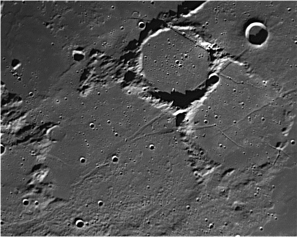
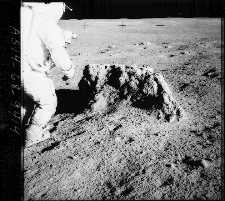
Friday, June 13 – Today in 1983, Pioneer 10 became the first man made object to leave the solar system. What wonders would it see? Are there other galaxies out there like our own? Will there be life like ours? While we can’t see through Pioneer’s “eyes,” tonight let’s take an historic journey to the Moon, as we look at the northeast shore of Mare Cognitum and the Apollo 14 mission landing site – Fra Mauro.

As craters go, 3.9 billion year old Fra Mauro is on the shallow side and spans 95 kilometers. At some 730 meters deep, standing at the foot of one of its walls would be like standing at the bottom of the Grand Canyon… Yet, time has so eroded this crater that its west wall is completely missing and its floor is covered with fissures.

NASA
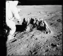
Even though ruined Fra Mauro seems like a forbidding place to land a manned mission, it remained high on the priority list because it is geologically rich. Ill-fated Apollo 13 was to land in a formation north of the crater which was formed by ejecta belonging to the Imbrium Basin – material which had already been mapped telescopically. By returning samples of this material from deep within the Moon’s crust, scientists would have been able to determine the exact time these changes came about.

As you view Fra Mauro tonight, picture yourself in a lunar rover traversing this barren landscape and viewing the rocks thrown out from a long-ago impact. How willing would you be to take on the vision of others and travel to another world?

Saturday, June 14 – As the day begins and you wait on dawn, keep watch for the peak of the Ophiuchid meteor shower with its radiant near Scorpius. The fall rate is poor with only three per hour, but fast moving bolides are common. Today is about the midpoint – and the activity peak – of this 25 day long stream.

Too moony to see anything? Then try an experiment both Ian and I have been working on. When a meteoroid enters our atmosphere, it has an impact on the ionosphere. Take a few moments and download Google Ionosphere and watch what happens as the meteor shower progresses! And don’t forget the “radio” either… Simply tune any FM radio to the lowest frequency that doesn’t receive a clear signal and listen. These ionospheric disturbances will sound like snatches of radio signal, hisses, pops and more. It’s a great way to catch a meteor shower with more than just your eyes!

Wes Higgins
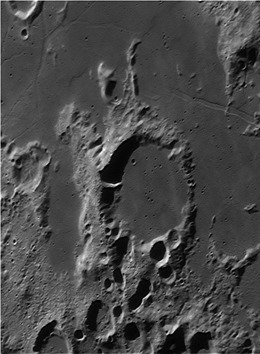
Tonight let’s venture toward the south shore of Palus Epidemiarum to have a high power look at crater Capuanus. Named for Italian astronomer Francesco Capuano di Manfredonia, this 60 kilometer wide crater boasts a still-tall southwest wall, but the northeast one was destroyed by lava flow. At its highest, it reaches around 1900 meters above the lunar surface, yet drops to no more than 300 meters at the lowest. Look for several strikes along the crater walls as well as more evidence of a strong geological history. To its north is the Hesiodus Rima…a huge fault line extending 300 kilometers across the surface!

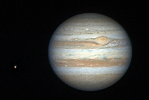
To the east, Jupiter is now rising… But give it some time to clear the atmospheric distortion! By far brighter than neighboring stars to the unaided eye, giant Jupiter will move slowly along the ecliptic plane over the course of the evening. To smaller binoculars it is easily observed as an orb with two grey bands across the middle. To larger binoculars, the equatorial belts become much clearer and the four Galilean moons are easily seen with steady hands. To the small telescope, no planet offers greater details. Even at very low magnifying power, the north, south and central equatorial zones are easily observable and all four moons are clear and steady.

Wes Higgins
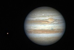
For most observers, tonight will show Callisto, Ganymede, Europa and Io grouped to the east of the Mighty Jove, but as time progresses, so do their positions! Try observing over a period of several hours and watch just how quickly these four bright moons shuttle around… You might even catch a possible transit of Io!

To the mid-sized telescope, far greater details begin to appear – such as temperate belts on the planet’s surface and the soft appearance of the Great Red Spot. Finer details are visible during steady seeing, and small things like being able to see which satellite is closer to – or further away from – our vantage point become very easy. Simple things, like watching a moon transit the surface and the resulting shadow on the planet are much easier. With a large telescope, seeing details on Jupiter depends more on seeing conditions. While more aperture allows finer views – conditions are everything when it comes to the Mighty Jove!

Wes Higgins
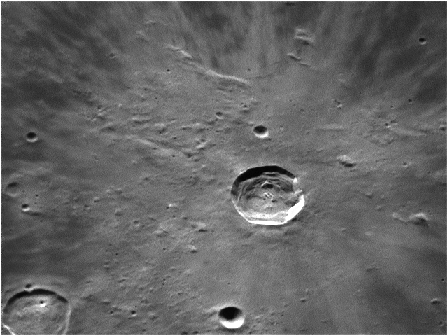
Sunday, June 15 – As we wait on the sky to darken tonight, let’s start our adventures by taking a close look at crater Kepler. Situated just north of central along tonight’s terminator, this great crater named for Johannes Kepler only spans 32 kilometers, but drops to a deep 2750 meters below the surface. This class I crater is a geological hotspot!

As the very first to be mapped by the U.S. Geological Survey, the area around Kepler contains many smooth lava domes reaching no more than 30 meters above the plains. According to records, in 1963 a glowing red area was spotted near Kepler and extensively photographed. Normally one of the brightest regions of the Moon, the brightness value at the time nearly doubled! Although it was rather exciting, scientists later determined the phenomenon was caused by high energy particles from a solar flare reflecting from Kepler’s high albedo surface. In the days ahead all details around Kepler will be lost, so take this opportunity to have a good look at one awesome small crater!

Palomar Observatory, courtesy of Cal Tech
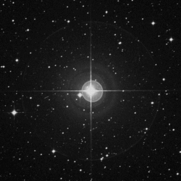
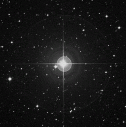
When skies are dark, it’s time to have a look at the 250 light-year distant silicon star Iota Librae (RA 15 12 13 Dec 19 47 28). This is a real challenge for binoculars – but not because the components are so close. In Iota’s case, the near 5th magnitude primary simply overshadows its 9th magnitude companion! In 1782, Sir William Herschel measured them and determined them to be a true physical pair. Yet, in 1940 Librae A was determined to have an equal magnitude companion only 0.2 arcseconds away… And the secondary was proved to have a companion of its own which echoes the primary. A four star system!

No matter if you stayed up late chasing deep sky, or got up early, right now is the time to catch the peak of the June Lyrids meteor shower. Although the Moon will make observing difficult, it’s still an opportunity for those wishing to log their meteor observations. Look for the radiant near bright Vega – you may see up to 15 faint blue meteors per hour from this branch of the May Lyrid meteor stream. Try the ionosphere and radio observing!!

Wishing you clear skies and a great weekend…

This week’s image credits: Detail view of Fra Mauro, Capuanus, Kepler and Jupiter – Credit: Wes Higgins, Shepard at Frau Mauro – Credit: NASA, Iota Librae – Credit: Palomar Observatory, courtesy of Caltech.

So, What Do Astronomers Do With A 55 Meter-Long Image?

The new 55-meter image that was unveiled today is impressive, but does it hold any scientific value? A resounding yes to that question came from astronomers who helped work on this project, and given the standing room only for the oral presentation of the scientific research going into this image, plenty of other astronomers are interested in the discoveries from Spitzer’s five-year effort of gathering infrared data of our home galaxy. “This is a legacy science project,” said Barbara Whitney of the Space Science Institute, “that shows star formation as never seen before on both the large and small scale. Most of these star forming regions are being seen for the first time.”

“This is the highest-resolution, largest, most sensitive infrared picture ever taken of our Milky Way,” said Sean Carey of NASA’s Spitzer Science Center. “Where previous surveys saw a single source of light, we now see a cluster of stars. With this data, we can learn how massive stars form, map galactic spiral arms and make a better estimate of our galaxy’s star-formation rate,” Carey explained.

From our vantage point on Earth, we see the Milky Way as a blurry, narrow band of light that stretches across the sky. In the visible, we only see about 5% of what’s actually out there. But with Spitzer’s dust-piercing infrared eyes, astronomers have peered 60,000 light-years away into this fuzzy band, called the galactic plane, and saw all the way to the other side of the galaxy.

The result is a cosmic tapestry depicting an epic coming-of-age tale for stars.

While evolved stars are seen as blue, the star forming regions are seen as green. The regions where young stars reside are revealed as “bubbles,” or curved ridges in the green clouds. These bubbles are carved by the winds from the outflow of dust from the young stellar objects. The starlets appear as yellow and red dots, and wisps of red are dust particles.

“With these Spitzer data, we’ve been able to catalogue more than 100 million stars,” said Edward Churchwell of the University of Wisconsin, at Madison.

“This picture shows us that our Milky Way galaxy is a crowded and dynamic place. We have a lot to learn. I’ve definitely found a lot of things in this map that I didn’t expect to see,” said Carey.

The A-Train: Using Five Satellites as One to Analyze Polluted Clouds

The A-Train - 5 satellites collaborate to scan polluted clouds (NASA)

This is one of the finest examples of satellite collaboration. Five Earth-observing orbiters, four from NASA and one from France, are working together to provide the deepest analysis of cloud cover ever carried out. The satellites orbit in a close formation, only eight minutes apart, and create what is known as the “Afternoon Constellation” (or “A-Train” for short). They are so close in fact, that they can be considered to act as one satellite, capable of carrying out a vast suite of measurements on the pollution content of clouds. This work is shedding new light on the link between clouds, pollution and rainfall, a study that could never be achieved with one satellite alone…

Pollution in clouds is a critical problem for the international community. These rogue particles can seriously change the natural behaviour of clouds and entire weather systems, but until now, scientists have been uncertain about the difference in rainfall from polluted and unpolluted cloud cover. This is primarily because no single environmental satellite has been able to probe deep into clouds with the limited number of instruments it can carry. But using the collective power of five independent satellites, scientists are beginning to unlock the secrets polluted clouds have been hiding.

Particulates from pollution mixing with clouds above the US (NASA)

Researchers at NASA’s Jet Propulsion Labs (JPL) in Pasadena have recently discovered that clouds peppered with pollutant particles do not produce as much rain as their unpolluted counterparts. This finding was only possible after analysing data from the near-simultaneous measurements made by the five A-Train satellites. The constellation includes NASA’s Aqua, Aura, CloudSat and CALIPSO and the French Space Agency’s PARASOL.

Typically, it is very hard to get a sense of how important the effect of pollution on clouds is. With the A-Train, we can see the clouds every day and we’re getting confirmation on a global scale that we have an issue here.” – Anne Douglass, project scientist at Goddard for NASA’s Aura satellite.

The A-Train is turning up some interesting, if alarming, results. When focusing on the skies above South America during the June-October dry season, the JPL team found that the increased level of agricultural burning during this period injected more aerosols into the clouds. This had the effect of shrinking the size of ice crystals in the clouds, preventing the crystals from getting large enough to fall as rain. This direct effect of burning and ice crystal formation has never been connected before the use of the A-Train. However, during wet seasons, the aerosol content in clouds appeared not to be a critical factor on the amount of rainfall.

How is it possible to distinguish between polluted and unpolluted clouds? Firstly, the A-Train’s Aura satellite measures the concentration of carbon monoxide in the clouds. This is a strong indicator for the presence of smoke and other aerosols originating from a power plant or agricultural activities. When the polluted clouds are identified, the A-Train’s Aqua satellite can be called into use. Using its Moderate Resolution Imaging Spectroradiometer instrument, the size of ice crystals in polluted and unpolluted clouds can be measured. Next up is NASA’s Tropical Rainfall Measuring Mission satellite that can measure the amount of precipitation (rain) from polluted and unpolluted clouds.

Through this combination of satellites, scientists are able to link pollution with clouds with precipitation. This is only one example of the flexibility behind collaborations such as A-Train, so cloud science can only go from strength to strength.

Source: Physorg.com

Solar Sonic Boom: Eclipses May Generate Atmospheric Shocks

The shadow of a lunar eclipse (NASA)

Something strange happens during a solar eclipse. As the Moon’s shadow passes over the surface of the Earth, observers have noticed mysterious bands of shadow ripple ahead and behind the eclipse. It seemed possible that these bands were a result of constructive and destructive interference of sunlight around the limb of the Moon (an effect known as diffraction), or atmospheric turbulence may have had a part to play. However, a new theory has come to light. As the Moon’s shadow travels across the Earth’s surface, it may be possible that the shadow cools the atmosphere suddenly, creating a pressure difference. This gives rise to a sonic phenomenon: a shock front. This may refract the path of light from the lunar limb and through the atmosphere, creating the bands of light and dark. The solar eclipse may be a sonic phenomenon as well as an optical one…

If an object travels faster than the speed of sound, a shock will form. This shock is generated as a body passes through the atmosphere faster than sound can propagate. On Earth, at sea level, the speed of sound is approximately 1,225 kilometres per hour (or 761 miles per hour; i.e. the sound of an explosion would take an hour to travel a distance of 761 miles). Should an aircraft travel at 1,225 km/hr or beyond, the pressure waves it generates cannot keep up with the plane. In this case, a shock wave will form, more commonly known as a “sonic boom” for stationary observers.

So, back to the solar eclipse. How can the shadow of the Moon create a sonic boom? It’s only a shadow, it’s not a solid body moving inside the atmosphere; surely a shock isn’t possible? Actually, research carried out by astrophysicist Dr Stuart Eves who works with the Surrey Satellite Technology Limited (SSTL) suggests it may be possible, and the phenomenon produced is known as “infrasound”. He believes that as the lunar shadow passes over the Earth’s surface, there is intense, local cooling of the atmosphere after the leading and before trailing edge of the eclipse. This cooling sets up a sudden pressure difference.

As the eclipse shadow moves through the atmosphere, the sudden disappearance of the Sun changes the Earth’s temperature.” – Dr Eves.

If we consider that the eclipse shadow travels at supersonic velocities (1,100 miles per hour at the equator and up to 5,000 miles per hour near the poles), and the strong pressure gradient travels with the eclipse, a shock front is created in the atmosphere, generating infrasound waves. The sub-audible infrasound generated by this occurrence modifies the atmosphere to such an extent that it will deflect the path of light through the atmosphere. In this case, the light and dark bands around the eclipse shadow would be created by refraction.

Some scientists are sceptical about this new theory, but Eves thinks his explanation may also help to explain other phenomena during eclipses. Infrasound may be responsible for strange Foucault pendulum behaviour (the sensitive pendulums – used to demonstrate the rotation of the Earth – swing wildly during eclipses). The infrasound pulses may cause the ground to vibrate, interfering with the pendulum swing. Infrasound may also explain some bizarre animal behaviour during these events. Sub audible sound wave frequencies are known to distress or alarm birds, perhaps their strange behaviour during eclipses could be down to infrasound propagation.

Source: BBC

More Satellite Images of China’s Earthquake

Beichuan Region of China, before and after Earthquake. Image credit: Formosat 2

More satellite images have been released portraying the devastation caused by the May 12, 2008 earthquake that struck China’s Sichaun Basin. This pair of images, captured by Taiwan’s Formosat-2, illustrates the challenges faced by rescuers bringing equipment and supplies to survivors of the massive 7.9-magnitude earthquake. The top “before” image from 2006 shows the tree-covered mountain terrain of China’s Beichuan County. A river curves along the base of the mountain, and a road follows the banks of the river.

In the lower image, taken on May 14, 2008, the landscape is almost unrecognizable. A landslide engulfed the entire mountainside, turning its green slopes brown. Both the road and the river are entirely gone, buried under the rubble, which rises in a mound up the opposite slope. Landslides, flooding and buckled roads have made travel within quake-affected regions difficult.


Landslides have created earthen dams, and new lakes were formed overnight. This pair of high-resolution images from Taiwan’s Formosat-2 satellite show a “before” and “after” comparison from May 14, 2006 (top),and May 14, 2008 (bottom.) Several landslides, a collapsed bridge, and a bridge submerged by a newly formed lake are visible in the “after” the earthquake image.


Finally, this bottom series of images show how devastation continues to occur as the earthquake and its aftershocks has sent earth and rock tumbling down mountains into rivers, creating natural dams behind which lakes quickly built up. The first, a “before” image taken in 2006, show normal springtime conditions.

On May 15, 2008, three days after the initial earthquake, both the bridge and the roads it connected had disappeared under murky water. Some sections of the villages remained above the waterline, as did portions of the roads leading to the villages. The tops of trees, perhaps on slightly higher ground, formed tiny islands near the shores of the growing lake.

Formosat-2 took the final image on May 19, 2008. By this time, water levels in the earthquake lake had risen enough to immerse both villages and the entire road network. Tan debris floats on the surface of the water, concentrated over the locations of the villages.

Earthquake-created dams present a dual danger. Apart from the upstream floods that occur as a lake builds behind the natural dam, the piles of rubble that form the dam may be unstable. Another quake or simply the pressure of water behind it could burst the dam, sending a wall of water downstream. Downstream floods may also occur when water begins to cascade over the top of the dam. Thousands of people were evacuated from Beichuan on May 17 when one such lake threatened to burst, said China Daily.

Original News Source: NASA’s Earth Observatory

Phytoplankton Bloom Erupts in the North Sea

Usually the North Sea conjures up cold and gloomy visions. But as the stunning image above shows, this isn’t always the case. ESA’s Envisat captured vast green swirls of phytoplankton bloom drifting in the North Sea currents on May 7th 2008; spring has most definitely sprung for the Scottish waters. But how is this bright green bloom produced? What has stirred up all this activity? It seems that for a short time, the lush green landscape of Fife is matched by the sea-faring plankton off the UK coast…

Phytoplankton through the microscope (NOAA)

This vivid green bloom was created by a type of plankton called phytoplankton. The microscopic plant floats near the surface of large bodies of water where sunlight is plentiful. Like any land-based plant, phytoplankton requires photosynthesis to survive. Other types of plankton include zooplankton (microscopic creatures) and bacterioplankton (water-borne bacteria) survive by feeding off other plankton varieties. The plant variety of plankton, phytoplankton, is well known to produce blooms when nutrients on the marine environment increase, boosting phytoplankton population. It would seem that the water off the Scotland coast has become particularly nutrient rich, with plenty of sunlight, creating magnificent displays observable from orbit.

Envisat above Earth (ESA)

This particular bloom was captured by the Medium Resolution Imaging Spectrometer (MERIS) instrument on board the ESA’s Envisat operating at a full spatial resolution of 300m (i.e. features of 300m can be resolved). The green hue is from the chlorophyll (essential for photosynthesis) contained within each phytoplankton cell. Depending on the phytoplankton species, it’s possible that there are hundreds to thousands of cells per millilitre of sea water.

Phytoplankton is very important when considering the concentrations of carbon dioxide in the atmosphere and their density in the worlds oceans are modelled in simulations of future climate change. During photosynthesis, they absorb carbon dioxide (and generate oxygen), so they form a highly influential carbon sink.

Source: ESA Picture of the Day

Satellite Images of China Earthquake

Some of the first satellite images have been released of areas in China hit by the 7.9 magnitude earthquake on May 12, 2008. This image shows Beichuan, one of the worst-hit areas in Sichuan Province of southwest China. The pictures reveal a large forest, a school and clusters of residential houses along a river that has been destroyed out by the quake. A road along the river was also severely damaged. The images were taken by Taiwan’s FORMOSAT-2 satellite. A “before” image is also available, taken in two years ago in May of 2006:

The pictures are expected to be used as references in China’s efforts in searching and rescuing people still missing in Sichuan.

Harry Chang, a professor of National Taiwan Normal University said the images have been given to the Chinese Academy of Sciences. Chang said that in Beichuan, the earthquake also caused landslides, evident in the top photo, covering some 1,500 hectares (3,705 acres), which had blocked the river.

“Accordingly, several new lakes have been formed. What is dangerous is that should the new lakes burst, the residents living in the low-lying areas of the river would be in danger,” he said.

Chang also warned of mudslides caused by rain, saying “it would make the rescue work more difficult.” As of May 15, officials estimated the death toll could reach 50,000.

Monday’s earthquake began at 2:28 p.m. local time (06:28 UTC). The quake was felt throughout much of China, as well as parts of Taiwan, Thailand, and Vietnam. This elevation map above shows the region where the earthquake struck. Green indicates the lowest elevations, and beige the highest. The data for this map were collected by NASA’s Shuttle Radar Topography Mission (SRTM) in 2000. Overlain onto the map are earthquake magnitude indicators. The earthquake’s epicenter was approximately 90 kilometers (55 miles) west-northwest of the city of Chengdu. Smaller magnitude events occurred northeast of the epicenter, and generally followed the edge of the Longmen Shan mountain range.

Original News Sources: The China Post, NASA Earth Observatory