It’s impossible to do an article about Uranus without opening up the back door to a spit storm of potty humour. I get it, there’s something just hilarious about talking about your, mine and everyone’s anus. And even if you use the more sanitized and sterile term urine-us, it’s still pretty dirty, in an unwashed New York stairwell kind of way. You’re in us? No.
This is a no-win solution. It’s a Kobayashi Maru scenario here. We’re all doomed.
Can we call a truce? I dare you commentators, to keep the YouTube comments as pure and clean as driven snow, so we can focus on the super interesting science. Think of the children.
Let’s set the stage, I’m going to let planetary astronomer Kevin Grazier give you the proper pronunciation to clear our minds and let us move forward with grace and civility.
Kevin Grazier:
Strictly speaking, it’s pronounced Youranous, is the pronunciation.
As you probably know, Uranus… I mean Ouranus. No, I can’t do it, my brainwashing is too far along. Save yourselves!. Anyway, Uranus is the 7th planet from the Sun, and the 3rd largest planet in the Solar System. Jupiter and Saturn get all the spacecraft and Hubble space telescopes, but Uranus is an incredibly worthwhile target to visit.
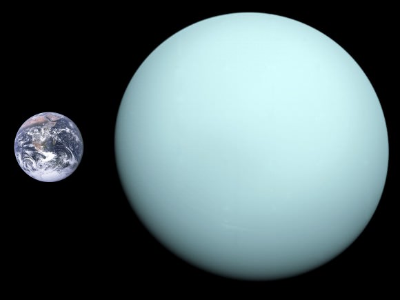
Diameter comparison of Uranus and Earth. Approximate scale is 90 km/px. Credit: NASA
It’s almost exactly 4 times larger than Earth and has its own set of strange dusty rings – perhaps left over from a shattered moon. It has at least 27 moons, that we know of, and many more interesting features that would fascinate astronomers, if we had a spacecraft there, which we don’t. Which is ridiculous. We’ve only made one close flyby of Uranus by Voyager II back in 1986.
We’ve seen Pluto up close, but there are no plans to visit Uranus? Madness.
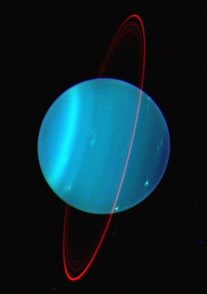
Credit: Lawrence Sromovsky, (Univ. Wisconsin-Madison), Keck Observatory.
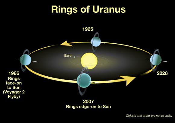
Anyway, perhaps one of the strangest aspects of Uranus is its tilt. The planet is flipped over on its side, like a Weeble, that wouldn’t unwobble.
Actually, all the planets in the Solar System have some level of axial tilt. The Earth is tilted 23.5 degrees away from the Sun’s equator. Mars is 25 degrees, and even Mercury is 2.1 degrees tilted. These tilts are everywhere.
But Uranus is 97.8 degrees. That’s just 0.2 degrees shy of a 90s boy band.
You might be wondering, why have it be more than 90 degrees. High school geometry tells me that 97.8 degrees is the same as 82.2 degrees. And that’s true. But astronomers define the angle as greater than 90 degrees when you take its direction of rotation into account. When you describe it as turning in the same direction as the rest of the planets in the Solar System, then you have to measure it this way.
What could have done that to Uranus, how could it have happened?
The fact that Uranus is flipped over on its side tells us that the calm clockwork motion of the Solar System hasn’t always been this way. Shortly after the formation of the Sun and planets, our neighborhood was a violent place.
The early planets smashed into each other, pushed one another into new orbits. Some planets could have been spun out of the Solar System entirely, while others might have been driven into the Sun. Our own Moon was likely formed when a Mars-sized object crashed into the Earth. Other moons might have been captured from three body interactions between worlds. It was mayhem.
The Solar System that you see today contains the survivors. Everything that wasn’t delivered a death blow.
And something really tried to deliver a death blow to Uranus, very early after it formed. We know this because the moons of Uranus orbit at the same tilt as the planet’s axis. This means that something smashed into Uranus while it was still surrounded by the disk of gas and dust that its moons formed from.
When the massive collision happened, the planet flipped over, wrenching this disk with it. The moons formed within this new configuration.
Astronomers think it was more complicated than that, however. If it was a single, massive collision, models suggest the planet would just flip over entirely, and end up rotating backwards from the other planets in the Solar System.
It’s more likely that another collision or even a series of collisions put the brakes on Uranus’ end over end roll, putting it into its current configuration. It boggles the mind to think about what must have happened.
Uranus’ tilt drastically affects the amount of sunlight the hemispheres receive during its orbit. Credit: NASA, ESA, and A. Feild (STScI)
Having such a huge axial tilt makes a big different to Uranus. As it travels around the Sun in its 84-year orbit, the planet still has its poles pointed at fixed locations in space. This means that it spends 42 years with its northern hemisphere roughly pointed towards the Sun, and 42 years with its southern hemisphere in sunlight.
If you could stand on the north pole of Uranus, the Sun would be directly overhead in the middle of summer, and then it would make bigger and bigger circles until it dipped below the horizon a few decades later. Then you wouldn’t see it for a few decades until it finally reappeared again. It would be very very strange.
Of course, it’s a gas planet, so you can’t stand on it. If you could stand on it, we’d all be marveling at your ability to stand on planets.
Here we are in our calm, ordered Solar System, everything’s business as usual. But if you look around, you realize it’s pretty amazing that our planet is even here. Poor sideways Uranus is a testament to our good luck.
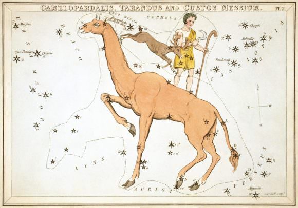
The large but faint northern Camelopardalis constellation (aka. "the giraffe"). Credit: astronoo.com
Welcome back to Constellation Friday! Today, in honor of our dear friend and contributor, Tammy Plotner, we examine the Caelum constellation. Enjoy!
In the 2nd century CE, Greek-Egyptian astronomer Claudius Ptolemaeus (aka. Ptolemy) compiled a list of the then-known 48 constellations. Until the development of modern astronomy, his treatise (known as the Almagest) would serve as the authoritative source on astronomy. This list has since come to be expanded to include the 88 constellations that are recognized by the International Astronomical Union (IAU) today.
One of these modern additions is Camelopardalis, otherwise known as “the giraffe”. Located in the northern sky, this large but faint constellation is the eighteenth largest in the night sky. It belongs to the Ursa Major family of constellations and is bordered by Draco, Ursa Minor, Cepheus, Cassiopeia, Perseus, Auriga, Lynx, and Ursa Major and should be considered circumpolar.
Name and Meaning:
There is no real mythology connected to Camelopardalis since it is considered a “modern” constellation. Due to the faintness of the stars associated with it, the early Greeks considered this area of the sky to be empty – or a desert. But based on its Latin name, it could be considered to be a long-necked animal with the neck of a camel and the spots of a panther – connected to the twelve labors of Hercules.
Camelopardalis as depicted in Urania’s Mirror, a set of constellation cards published in London c.1825. Credit: Sidney Hall/Library of Congress
The true nature of the “giraffe,” unfortunately, remains unclear. However, the name could be a reference to the book of Genesis in the Bible. a theory that is based on the fact that when Jacob Bartsch included Camelopardalis on his star map of 1624, he described the constellation as a camel on which Rebecca rode into Canaan. But since Camelopardalis represents a giraffe, not a camel, this explanation is not considered likely.
Notable Features:
Beta Camelopardalis is the brightest star in this constellation. It is a binary star with a yellow G-type supergiant as the primary and is located approximately 1,000 light years from Earth. Beta Cam is also an X-ray source, which suggests that it undergoes some kind of solar-like magnetic behavior (which accounts for its periodic flashes).
Camelopardalis’ second brightest star is CS Camelopardalis, another binary located approximately 3,000 light years away. It consists of a blue-white B-type supergiant that exhibits non-radial pulsations (which means that some portions of the star’s surface expand while others contract). It has a magnitude 8.7 companion located 2.9 arcseconds away, and the entire system is located in the reflection nebula vdB 14.
Then there’s Sigma 1694 Camelopardalis (aka. Struve 1694), which represents the “head’ of the giraffe. This binary star is composed of a white A-type subgiant located 300 light years from Earth, and a spectroscopic binary that consists of two A-type main sequence stars. Then there’s VZ Camelopardalis, a semi-regular variable M-type red giant located approximately 470 light years from Earth.
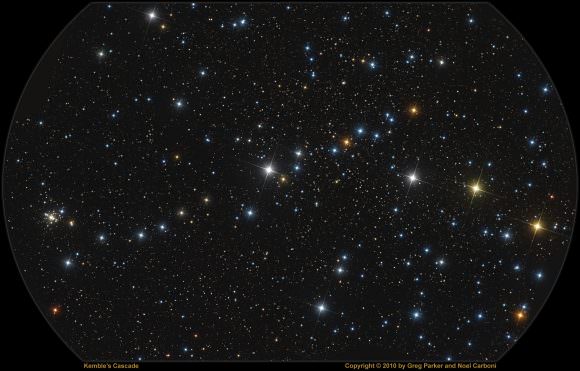
The asterism Kemble’s Cascade, located in the Camelopardalis constellation. Credit & Copyright: Noel Carboni/Greg Parker/New Forest Observatory/NASA
Camelopardalis is home to the asterism known as Kemble’s Cascade. Named after Father Lucian J. Kemble, a Franciscan Friar who discovered it, this asterism is formed by more than 20 stars that vary between magnitude 5 and 10 and form a straight line in the sky. After describing it to Walter Scott Houston (of Sky and Telescope magazine), Houston named it after Father Kemble and included it in his “Deep Sky Wonders” column in 1980.
Since Camelopardalis faces away from the galactic plane, a number of Deep Sky Objects are visible within its borders. These include NGC 2403, an intermediate spiral galaxy located approximately 12 million light years away. It was first discovered in the 18th century by William Herschel while he was working in England.
Then there’s NGC 1569, an irregular dwarf galaxy that is approximately 11 million light years away. This galaxy is known for the super star clusters it contains, both of which experience a considerable amount of star-forming activity. Then there’s NGC 1502, an open star cluster that is associated with Kemble’s Cascade and is located around 3,000 light years from Earth. NGC 1501, a planetary nebula, is located 1.4 degrees south of NGC 1502.
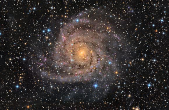
Camelopardalis is also home to IC 342, another intermediate spiral galaxy that is approximately 10.7 million light years away. It is one of the two brightest galaxies in the IC 342/Maffei Group (the nearest group of galaxies to the Local Group) and was discovered in 1895 by the British astronomer William Frederick Denning.
The spiral galaxy IC 342, located in the Camelopardalis constellation. Credit & Copyright: Stephen Leshin/NASA
History of Observation:
Camelopardalis was first recorded by Jakob Bartsch in 1624 but was most likely created by Petrus Plancius in 1613. Camelopardalis is the eighteenth largest constellation in the night sky, and its brightest stars are of the fourth magnitude. It was German astronomer Johannes Hevelius who gave it the official name of “Camelopardus” (alternately “Camelopardalis”) because he saw the constellation’s many faint stars as the spots of a giraffe.
Some of the stars in this constellation were used by William Croswell to form the constellation Sciurus Volans in 1810. However, this did not catch on with later cartographers. Today, Camelopardalis is one of the 88 constellations used by the IAU.
Finding Camelopardalis:
Located Camelopardalis is not too difficult a task, given its proximity to several major constellations. However, it is quite faint compared to its immediate neighbors, so good viewing conditions (low light pollution) are a plus. One of the easiest ways is to locate the Big Dipper (Ursa Major) in the night sky, then tracing from the tip of the “spoon” directly outwards towards the head of the bear.
Next, locate Cassiopeia on the other side of the night sky – easily identified by its characteristic W shape. Camelopardalis is directly between them and is identifiable by the three stars (alpha, beta, gamma) that form the “neck” of the giraffe. For those who know its coordinates, it is located in the second quadrant of the northern hemisphere (NQ2) and can be seen at latitudes between +90° and -10°.
With 36 stars that have Bayer/Flamsteed designations, Camelopardalis provides many opportunities for star gazing. Using binoculars, Alpha Cam can be spotted. This rare, blue-white class O super giant may very well be a runaway star that originated from the associated cluster NGC 1502. It appears faint because it is dimmed by nearly a full magnitude by intervening interstellar dust, and its true luminosity might be as much as 530,000 times that of our Sun.
Now take a look at slightly brighter Beta. At 40 million years old and about 1000 light years from our solar system, Beta has a mass of about 7 times greater than our Sun. But lying just over an arc minute away is a companion star which is in itself a double star that takes at least a million years to orbit the super giant parent star! According to Jim Kaler, Beta Cam is also a double mystery, one which is most likely making the transition from a hydrogen-fusing dwarf (of hot class B) to a larger helium-fusing red giant.
Whatever its status, it falls into a zone of temperature and luminosity in which stars become unstable and pulsate as Cepheid variable stars. Beta Cam, however, does not vary, though some multiple pulsations are present with periods of tens of days. During aircraft observations of meteors in 1967, Beta Cam was seen suddenly to flash, brightening by about a full magnitude over the course of a quarter of a second. So keep your eye on it… If you can find it!
For larger binoculars and small telescopes, check out NGC 1502. This small open cluster of approximately 45 stars is made even better by its proximity to an asterism known as “Kemble’s Cascade”. To find it, simply look around Polaris in a counterclockwise rotation moving outward by a field twice. It is two full binocular fields from Alpha and Beta. The cluster itself is very attractive, but look closely in the telescope, and you will see it also contains two double stars – Struve 484 and Struve 485!
Larger binoculars and small telescopes will also have no problem picking up NGC 2403 from a dark sky location. NGC 2403 is a spiral galaxy discovered by William Herschel that belongs to the M81 galaxy group. At around 8 million light-years from Earth, larger telescopes will notice the northern spiral arm connects to NGC 2404 in a satellite galaxy interaction. Allan Sandage detected Cepheid variables in NGC 2403 using the Hale telescope, making it the first galaxy beyond our local group to have Cepheids found in it. As of late 2004, there had been two reported supernovae in the galaxy.
For larger telescopes and an observing challenge, try planetary nebula NGC 1501. Discovered in 1787 by Sir William Herschel and located about 4,890 light years away, this irregular disc has a great 14th magnitude central star hidden inside the dimpled structure, which gives rise to its popular moniker – the “Oyster Nebula.” Find the pearl!
For a dim fuzzy, hunt down NGC 2715. At magnitude 13.6, this small barred spiral galaxy may have recently experienced a galaxy merger, and as many as three supernovae events have been detected recently. For a true test of your observing skills and equipment, try IC 342. IC 342 is a nearby giant spiral that has a significant dust light extinction. It averages about magnitude 9, and it’s quite large (20′).
Once you’ve found it, see if you can spot its very stellar nucleus. While the exact size and mass of this galaxy are still the subject of controversy, there are strong indications that in many respects, IC 342 resembles a giant spiral (similar to our own Galaxy) and competes with two other near giant spirals – the Milky Way and Andromeda (M 31) – for the gravitational influence in the Local Volume.
There is one meteor shower associated with the constellation of Camelopardalis – the March Camelopardalids. They occur on or about March 22nd with no definite peak, and the fall rate averages only about one per hour. They are the slowest known meteors at 7 kps.
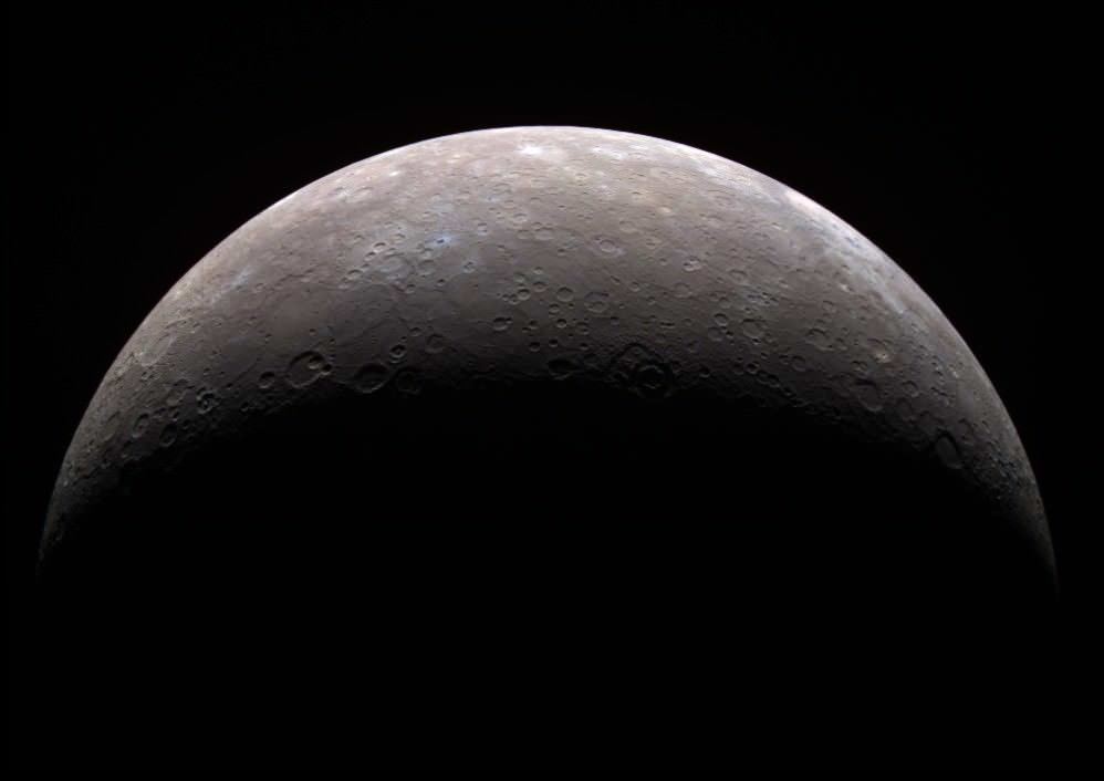
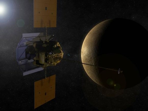
Planet Mercury as seen from the MESSENGER spacecraft in 2008. Credit: NASA/JPL
Welcome back to the first in our series on Settling the Solar System! First up, we take a look at that hot, hellish place located closest to the Sun – the planet Mercury!
Humanity has long dreamed of establishing itself on other worlds, even before we started going into space. We’ve talked about colonizing the Moon, Mars, and even establishing ourselves on exoplanets in distant star systems. But what about the other planets in our own backyard? When it comes to the Solar System, there is a lot of potential real estate out there that we don’t really consider.
Well, consider Mercury. While most people wouldn’t suspect it, the closest planet to our Sun is actually a potential candidate for settlement. Whereas it experiences extremes in temperature – gravitating between heat that could instantly cook a human being to cold that could flash-freeze flesh in seconds – it actually has potential as a starter colony.
Examples in Fiction:
The idea of colonizing Mercury has been explored by science fiction writers for almost a century. However, it has only been since the mid-20th century that colonization has been dealt with in a scientific fashion. Some of the earliest known examples of this include the short stories of Leigh Brackett and Isaac Asimov during the 1940s and 50s.
In the former’s work, Mercury is a tidally-locked planet (which was what astronomers believed at the time) that has a “Twilight Belt” characterized by extremes in heat, cold, and solar storms. Some of Asimov’s early work included short stories where a similarly tidally-locked Mercury was the setting, or characters came from a colony located on the planet.
Mercury, as imaged by the MESSENGER spacecraft, revealing parts of the never seen by human eyes. Credit: NASA/Johns Hopkins University Applied Physics Laboratory/Carnegie Institution of Washington
These included “Runaround” (written in 1942, and later included in I, Robot), which centers on a robot that is specifically designed to cope with the intense radiation of Mercury. In Asimov’s murder-mystery story “The Dying Night” (1956) – in which the three suspects hail from Mercury, the Moon, and Ceres – the conditions of each location are key to finding out who the murderer is.
In 1946, Ray Bradbury published “Frost and Fire”, a short story that takes place on a planet described as being next to the sun. The conditions on this world allude to Mercury, where the days are extremely hot, the nights extremely cold, and humans live for only eight days. Arthur C. Clarke’s Islands in the Sky (1952) contains a description of a creature that lives on what was believed at the time to be Mercury’s permanently dark side and occasionally visits the twilight region.
In his later novel, Rendezvous with Rama (1973), Clarke describes a colonized Solar System which includes the Hermians, a toughened branch of humanity that lives on Mercury and thrives off the export of metals and energy. The same setting and planetary identities are used in his 1976 novel Imperial Earth.
In Kurt Vonnegut’s novel The Sirens of Titan (1959), a section of the story is set in caves located on the dark side of the planet. Larry Niven’s short story “The Coldest Place” (1964) teases the reader by presenting a world that is said to be the coldest location in the Solar System, only to reveal that it is the dark side of Mercury (and not Pluto, as is generally assumed).
“Lava Falls on Mercury” (by Ken Fagg) for If magazine, June 1954. Credit: Public Domain
Mercury also serves as a location in many of Kim Stanley Robinson’s novels and short stories. These include The Memory of Whiteness (1985), Blue Mars (1996), and 2312 (2012), in which Mercury is the home to a vast city called Terminator. To avoid the harmful radiation and heat, the city rolls around the planet’s equator on tracks, keeping pace with the planet’s rotation so that it stays ahead of the Sun.
In 2005, Ben Bova published Mercury (part of his Grand Tour series) that deals with the exploration of Mercury and colonizing it for the sake of harnessing solar energy. Charles Stross’ 2008 novel Saturn’s Children involves a similar concept to Robinson’s 2312, where a city called Terminator traverses the surface on rails, keeping pace with the planet’s rotation.
Proposed Methods:
A number of possibilities exist for a colony on Mercury, owing to the nature of its rotation, orbit, composition, and geological history. For example, Mercury’s slow rotational period means that one side of the planet is facing towards the Sun for extended periods of time – reaching temperatures highs of up to 427 °C (800 °F) – while the side facing away experiences extreme cold (-193 °C; -315 °F).
In addition, the planet’s rapid orbital period of 88 days, combined with its sidereal rotation period of 58.6 days, means that it takes roughly 176 Earth days for the Sun to return to the same place in the sky (i.e. a solar day). Essentially, this means that a single day on Mercury lasts as long as two of its years. So if a city were placed on the night-side, and had tracks wheels so it could keep moving to stay ahead of the Sun, people could live without fear of burning up.
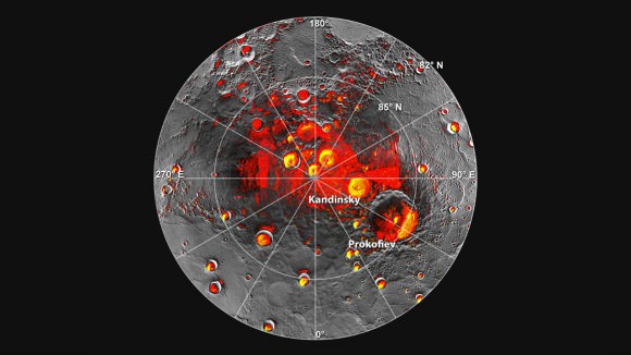
Images of Mercury’s northern polar region, provided by MESSENGER. Credit: NASA/JPL
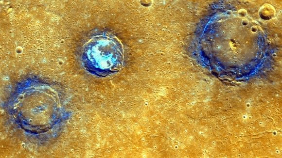
In addition, Mercury’s very low axial tilt (0.034°) means that its polar regions are permanently shaded and cold enough to contain water ice. In the northern region, a number of craters were observed by NASA’s MESSENGER probe in 2012 which confirmed the existence of water ice and organic molecules. Scientists believe that Mercury’s southern pole may also have ice, and claim that an estimated 100 billion to 1 trillion tons of water ice could exist at both poles, which could be up to 20 meters thick in places.
In these regions, a colony could be built using a process called “paraterraforming” – a concept invented by British mathematician Richard Taylor in 1992. In a paper titled “Paraterraforming – The Worldhouse Concept”, Taylor described how a pressurized enclosure could be placed over the usable area of a planet to create a self-contained atmosphere. Over time, the ecology inside this dome could be altered to meet human needs.
In the case of Mercury, this would include pumping in a breathable atmosphere, and then melting the ice to create water vapor and natural irrigation. Eventually, the region inside the dome would become a livable habitat, complete with its own water cycle and carbon cycle. Alternately, the water could be evaporated, and oxygen gas created by subjecting it to solar radiation (a process known as photolysis).
Another possibility would be to build underground. For years, NASA has been toying with the idea of building colonies in stable, underground lava tubes that are known to exist on the Moon. And geological data obtained by the MESSENGER probe during flybys it conducted between 2008 and 2012 led to speculation that stable lava tubes might exist on Mercury as well.
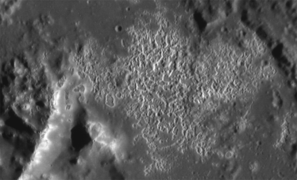
A previous MESSENGER image of hollows inside Tyagaraja crater. Credit: NASA/Johns Hopkins University Applied Physics Laboratory/Carnegie Institution of Washington
This includes information obtained during the probe’s 2009 flyby of Mercury, which revealed that the planet was a lot more geologically active in the past than previously thought. In addition, MESSENGER began spotting strange Swiss cheese-like features on the surface in 2011. These holes, which are known as “hollows”, could be an indication that underground tubes exist on Mercury as well.
Colonies built inside stable lava tubes would be naturally shielded to cosmic and solar radiation, extremes in temperature, and could be pressurized to create breathable atmospheres. In addition, at this depth, Mercury experiences far less in the way of temperature variations and would be warm enough to be habitable.
Potential Benefits:
At a glance, Mercury looks similar to the Earth’s Moon, so settling it would rely on many of the same strategies for establishing a moon base. It also has abundant minerals to offer, which could help move humanity towards a post-scarcity economy. Like Earth, it is a terrestrial planet, which means it is made up of silicate rocks and metals that are differentiated between an iron core and silicate crust and mantle.
However, Mercury is composed of 70% metals whereas’ Earth’s composition is 40% metal. What’s more, Mercury has a particular large core of iron and nickel, and which accounts for 42% of its volume. By comparison, Earth’s core accounts for only 17% of its volume. As a result, if Mercury were to be mined, enough minerals could be produced to last humanity indefinitely.
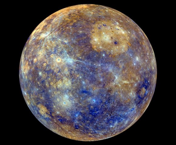
The different colors in this MESSENGER image of Mercury indicate the planet’s chemical, mineralogical, and physical differences. Credit: NASA/Johns Hopkins University Applied Physics Laboratory/Carnegie Institution of Washington.
Its proximity to the Sun also means that it could harness a tremendous amount of energy. This could be gathered by orbital solar arrays, which would be able to harness energy constantly and beam it to the surface. This energy could then be beamed to other planets in the Solar System using a series of transfer stations positioned at Lagrange Points.
Also, there’s the matter of Mercury’s gravity, which is 38% percent of Earth’s gravity. This is over twice what the Moon experiences, which means colonists would have an easier time adjusting to it. At the same time, it is also low enough to present benefits as far as exporting minerals is concerned, since ships departing from the surface would need less energy to achieve escape velocity.
Lastly, there is the distance to Mercury itself. At an average distance of about 93 million km (58 million mi), Mercury ranges between being 77.3 million km (48 million mi) to 222 million km (138 million mi) away from the Earth. This puts it a lot closer than other possible resource-rich areas like the Asteroid Belt (329 – 478 million km distant), Jupiter and its system of moons (628.7 – 928 million km), or Saturn’s (1.2 – 1.67 billion km).
Also, Mercury achieves inferior conjunction – the point where it is at its closest point to Earth – every 116 days, which is significantly shorter than either Venus’ or Mars’. Basically, missions destined for Mercury could launch almost every four months, whereas launch windows to Venus and Mars would have to take place every 1.6 years and 26 months, respectively.
The MESSENGER spacecraft has been in orbit around Mercury since March 2011 – but its days are numbered. Credit: NASA/JHUAPL/Carnegie Institution of Washington
In terms of travel time, several missions have been mounted to Mercury that can give us a ballpark estimate of how long it might take. For instance, the first spacecraft to travel to Mercury, NASA’s Mariner 10 spacecraft (which launched in 1973), took about 147 days to get there.
More recently, NASA’s MESSENGER spacecraft launched on August 3rd, 2004 to study Mercury in orbit, and made its first flyby on January 14th, 2008. That’s a total of 1,260 days to get from Earth to Mercury. The extended travel time was due to engineers seeking to place the probe in orbit around the planet, so it needed to proceed at a slower velocity.
Challenges:
Of course, a colony on Mercury would still be a huge challenge, both economically and technologically. The cost of establishing a colony anywhere on the planet would be tremendous and would require abundant materials to be shipped from Earth, or mined on site. Either way, such an operation would require a large fleet of spaceships capable of making the journey in a respectable amount of time.
Such a fleet does not yet exist, and the cost of developing it (and the associated infrastructure for getting all the necessary resources and supplies to Mercury) would be tremendous. Relying on robots and in-situ resource utilization (ISRU) would certainly cut costs and reduce the amount of materials that would need to be shipped. But these robots and their operations would need to be shielded from radiation and solar flares until they got the job done.
Enhanced-color image of Munch, Sander, and Poe craters amid volcanic plains (orange) near Caloris Basin. Credit: NASA/Johns Hopkins University Applied Physics Laboratory/Carnegie Institution of Washington
Basically, the situation is like trying to establish a shelter in the middle of a thunderstorm. Once it is complete, you can take shelter. But in the meantime, you’re likely to get wet and dirty! And even once the colony was complete, the colonists themselves would have to deal with the ever-present hazards of radiation exposure, decompression, and extremes in heat and cold.
As such, if a colony was established on Mercury, it would be heavily dependent on its technology (which would have to be rather advanced). Also, until such time as the colony became self-sufficient, those living there would be dependent on supply shipments that would have to come regularly from Earth (again, shipping costs!)
Still, once the necessary technology was developed, and we could figure out a cost-effective way to create one or more settlements and ship to Mercury, we could look forward to having a colony that could provide us with limitless energy and minerals. And we would have a group of human neighbors known as Hermians!
As with everything else pertaining to colonization and terraforming, once we’ve established that it is in fact possible, the only remaining question is “how much are we willing to spend?”
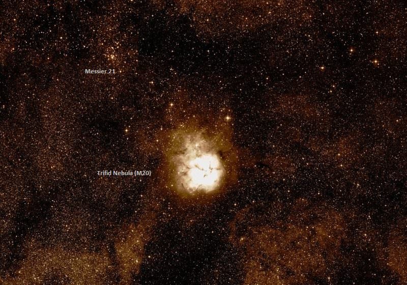
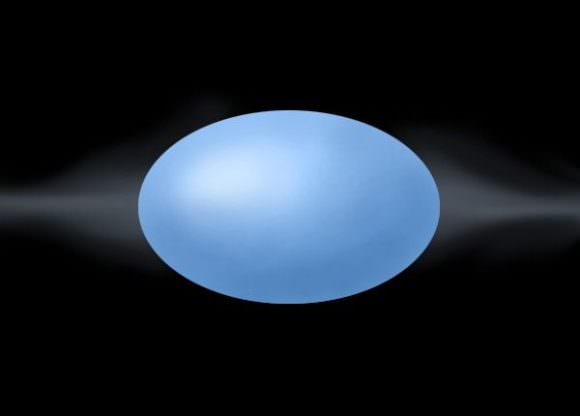
The Messier 21 open star cluster and the Trifid Nebula. Credit: Wikisky
Welcome back to Messier Monday! In our ongoing tribute to the great Tammy Plotner, we take a look at the Messier 21 open star cluster. Enjoy!
Back in the 18th century, famed French astronomer Charles Messier noted the presence of several “nebulous objects” in the night sky. Having originally mistaken them for comets, he began compiling a list of these objects so that other astronomers wouldn’t make the same mistake. Consisting of 100 objects, the Messier Catalog has come to be viewed as a major milestone in the study of Deep Space Objects.
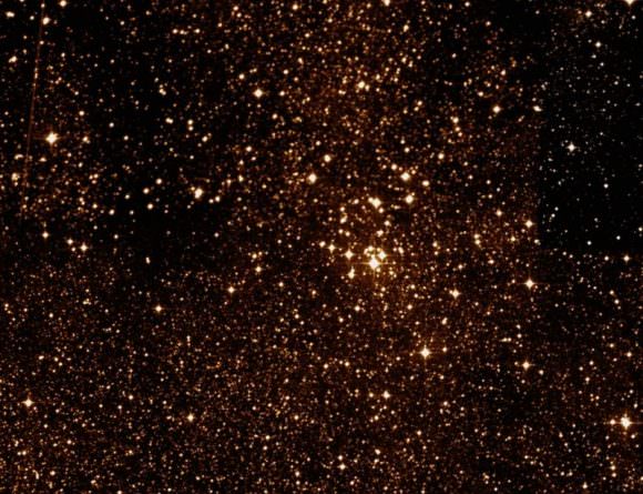
One of these objects is Messier 21 (aka. NGC 6531), an open star cluster located in the Sagittarius constellation. A relatively young cluster that is tightly packed, this object is not visible to the naked eye. Hence why it was not discovered until 1764 by Charles Messier himself. It is now one of the over 100 Deep Sky Objects listed in the Messier Catalog.
Description:
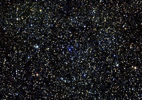
At a distance of 4,250 light years from Earth, this group of 57 various magnitude stars all started life together about 4.6 million years ago as part of the Sagittarius OB1 stellar association. What makes this fairly loose collection of stars rather prized is its youth as a cluster, and the variation of age in its stellar members. Main sequence stars are easy enough to distinguish in a group, but low mass stars are a different story when it comes to separating them from older cluster members.
Atlas mosaic image of Messier 21 (NGC 6531) obtained as part of the Two Micron All Sky Survey (2MASS). Credit: 2MASS/UofM/IPAC/Catech/NASA/NSF
As Byeong Park of the Korean Astronomy Observatory said in a 2001 study of the object:
“In the case of a young open cluster, low-mass stars are still in the contraction phase and their positions in the photometric diagrams are usually crowded with foreground red stars and reddened background stars. The young open cluster NGC 6531 (M21) is located in the Galactic disk near the Sagittarius star forming region. The cluster is near to the nebula NGC 6514 (the Trifid nebula), but it is known that it is not associated with any nebulosity and the interstellar reddening is low and homogeneous. Although the cluster is relatively near, and has many early B-type stars, it has not been studied in detail.”
But study it in detail they did, finding 56 main sequence members, 7 pre-main sequence stars and 6 pre-main sequence candidates. But why did this cluster… you know, cluster in the way it did? As Didier Raboud, an astronomer from the Geneva Observatory, explained in his 1998 study “Mass segregation in very young open clusters“:
“The study of the very young open cluster NGC 6231 clearly shows the presence of a mass segregation for the most massive stars. These observations, combined with those concerning other young objects and very recent numerical simulations, strongly support the hypothesis of an initial origin for the mass segregation of the most massive stars. These results led to the conclusion that massive stars form near the center of clusters. They are strong constraints for scenarii of star and stellar cluster formation.” say Raboud, “In the context of massive star formation in the center of clusters, it is worth noting that we observe numerous examples of multiple systems of O-stars in the center of very young OCs. In the case of NGC 6231, 8 stars among the 10 brightest are spectroscopic binaries with periods shorter than 6 days.”
Achernar, the flattest star known, is classified as be star. Credit: earthsky.org
“Be stars are a class of rapidly rotating B stars with circumstellar disks that cause Balmer and other line emission. There are three possible reasons for the rapid rotation of Be stars: they may have been born as rapid rotators, spun up by binary mass transfer, or spun up during the main-sequence (MS) evolution of B stars. To test the various formation scenarios, we have conducted a photometric survey of 55 open clusters in the southern sky. We use our results to examine the age and evolutionary dependence of the Be phenomenon. We find an overall increase in the fraction of Be stars with age until 100 Myr, and Be stars are most common among the brightest, most massive B-type stars above the zero-age main sequence (ZAMS). We show that a spin-up phase at the terminal-age main sequence (TAMS) cannot produce the observed distribution of Be stars, but up to 73% of the Be stars detected may have been spun-up by binary mass transfer. Most of the remaining Be stars were likely rapid rotators at birth. Previous studies have suggested that low metallicity and high cluster density may also favor Be star formation.”
History of Observation:
Charles Messier discovered this object on June 5th, 1764. As he wrote in his notes on the occassion:
“In the same night I have determined the position of two clusters of stars which are close to each other, a bit above the Ecliptic, between the bow of Sagittarius and the right foot of Ophiuchus: the known star closest to these two clusters is the 11th of the constellation Sagittarius, of seventh magnitude, after the catalog of Flamsteed: the stars of these clusters are, from the eighth to the ninth magnitude, environed with nebulosities. I have determined their positions. The right ascension of the first cluster, 267d 4′ 5″, its declination 22d 59′ 10″ south. The right ascension of the second, 267d 31′ 35″; its declination, 22d 31′ 25″ south.”
Close up of the Messier 21 star cluster. Credit: Wikisky
While Messier did separate the two star clusters, he assumed the nebulosity of M20 was also involved with M21. In this circumstance, we cannot fault him. After all, his job was to locate comets, and the purpose of his catalog was to identify those objects that were not. In later years, Messier 21 would be revisited again by Admiral Smyth, who would describe it as follows:
“A coarse cluster of telescopic stars, in a rich gathering galaxy region, near the upper part of the Archer’s bow; and about the middle is the conspicuous pair above registered, – A being 9, yellowish, and B 10, ash coloured. This was discovered by Messier in 1764, who seems to have included some bright outliers in his description, and what he mentions as nebulosity, must have been the grouping of the minute stars in view. Though this was in the power of the meridian instruments, its mean apparent place was obtained by differentiation from Mu Sagittarii, the bright star about 2 deg 1/4 to the north-east of it.”
Locating Messier 21:
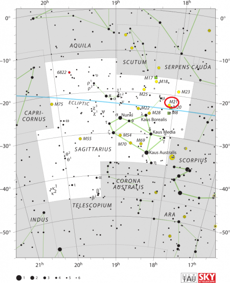
Once you have become familiar with the Sagittarius region, finding Messier 21 is easy. It’s located just two and a half degrees northwest of Messier 8 – the “Lagoon Nebula” – and about a half a degree northeast of Messier 20 – the “Trifid Nebula“. If you are just beginning to astronomy, try starting at the teapot’s tip star (Lambda) “Al Nasl”, and starhopping in the finderscope northwest to the Lagoon.
The location of M21 in the Sagittarius constellation. Credit: IAU/Sky & Telescope magazineRoger Sinnott & Rick Fienberg
While the nebulosity might not show in your finder, optical double 7 Sagittari, will. From there you will spot a bright cluster of stars two degrees due north. These are the stars embedded withing the Trifid Nebula, and the small, compressed area of stars to its northeast is the open star cluster M21. It will show well in binoculars under most sky conditions as a small, fairly bright concentration and resolve well for all telescope sizes.
And here are the quick facts, for your convenience:
Object Name: Messier 21 Alternative Designations: M21, NGC 6531 Object Type: Open Star Cluster Constellation: Sagittarius Right Ascension: 18 : 04.6 (h:m) Declination: -22 : 30 (deg:m) Distance: 4.25 (kly) Visual Brightness: 6.5 (mag) Apparent Dimension: 13.0 (arc min)
the southern constellation Caelum. Credit: absoluteaxarquia.com
Welcome back to Constellation Friday! Today, in honor of our dear friend and contributor, Tammy Plotner, we examine the Caelum constellation. Enjoy!
In the 2nd century CE, Greek-Egyptian astronomer Claudius Ptolemaeus (aka. Ptolemy) compiled a list of the then-known 48 constellations. Until the development of modern astronomy, his treatise (known as the Almagest) would serve as the authoritative source on astronomy. This list has since come to be expanded to include the 88 constellation that are recognized by the International Astronomical Union (IAU) today.
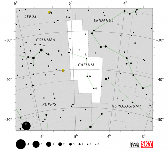
One of these constellations is Caelum, which was discovered in in the 1750s by French astronomer Nicolas Louis de Lacaille, and is now counted among the 88 IAU-recognized constellations. It is the eight-smallest constellation, with an area just less than that of Corona Australis (another southern constellation), and is bordered by the Dorado, Pictor, Horologium, Eridanus, Lepus and Columba constellations.
Name and Meaning:
The name Caelum, in Latin, literally means “chisel”, though the word can also mean ‘the heavens’. According to an antiquated school of thought, the sky (caelum, ‘sky, heaven, the heavens’) is rounded, spinning, and burning; and the sky is called by its name because it has the figures of the constellations impressed into it – just like an engraved (caelare) vessel. In Lacaille’s imagination, he saw this constellation as therefore representing “les Burins”, or the tools of a sculptor.
IAU map showing the location of the southern Caelum Constellation. Credit: IAU and Sky&Telescope magazine
Notable Features:
The constellation of Caelum has very little to offer observers using either binoculars or telescopes, with only four primary stars visible to the unaided eye and only eight stars with Bayer/Flamsteed designations. However, Gamma Caeli is a widely separated binary star system with a distance of 0.22°. It is composed of a magnitude 4.5 red giant and a magnitude 6.34 white giant.
For an extreme challenge, try locating Alpha Caeli. At an approximate distance of 65.7 light years from Earth, this yellow-white F-type main sequence dwarf with an apparent magnitude of +4.44 has an an extremely faint companion. It is magnitude 13, with a position angle of 121º and a separation 6.6″.
If you like long-term variable stars, you could always look for R Caeli, a long-term Mira-type that ranges from from 6.7 to 13.7 every 391 days. Or how about X Caeli, a Delta-Scuti type star? It’s changes are much faster – but far less noticeably. It changes by one tenth of a magnitude (6.3 to 6.4) every three hours and fourteen minutes.
For those looking for Deep Sky Objects, a big telescope is necessary. This is because NGC 1679 is about all there is to see, and it doesn’t appear lightly. Located about two degree south of Zeta Caeli, there’s not even a magnitude guess at this small spiral galaxy – but it does measure about 3.2 arc minutes, and appears to be an irregularly-shaped galaxy. There are indications that it may be a dwarf starburst galaxy.
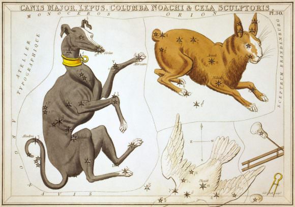
The Caleum constellation, depicted as “Cela Sculptoris” in the lower right of this 1825 star chart from Urania’s Mirror. Credit: Sidney Hall/Library of Congress
History of Observation:
Caelum was introduced by Nicolas Louis de Lacaille in the 1750s to help chart the southern hemisphere skies. Lacaille gave the constellation the French name Burin, which was originally Latinized to Caelum Scalptorium (“The Engravers’ Chisel”). English astronomer Francis Baily would alter shorten this name to Caelem, as suggested by fellow astronomer John Herschel.
In Lacaille’s original chart, the constellation was shown both as two types of chisels – a burin (a steel-engraving chisl) and an échoppe (an etching chisel) – although it has come to be recognized simply as a chisel.
Finding Caelum:
Though it is quite small and faint, locating Caelum is not difficult if you know where to look. Using stellar coordinates, you can find it by looking to the first quadrant of the southern hemisphere (SQ1), and then tracing it to between latitudes +40° and -90°. Or, start by picking out Canopus (the brightest of Carina‘s stars), pan due east, and then spot the small chisel between its neighbors.
Caelum is bordered by Dorado and Pictor to the south, Horologium and Eridanus to the east, Lepus to the north, and Columba to the west. The Caelum constellation occupies an area of 125 square degrees, and can be seen during the month of January at around 9 pm.
A depiction of the atomic structure of the helium atom. Credit: Creative Commons
Atomic theory has come a long way over the past few thousand years. Beginning in the 5th century BCE with Democritus‘ theory of indivisible “corpuscles” that interact with each other mechanically, then moving onto Dalton’s atomic model in the 18th century, and then maturing in the 20th century with the discovery of subatomic particles and quantum theory, the journey of discovery has been long and winding.
Arguably, one of the most important milestones along the way has been Bohr’ atomic model, which is sometimes referred to as the Rutherford-Bohr atomic model. Proposed by Danish physicist Niels Bohr in 1913, this model depicts the atom as a small, positively charged nucleus surrounded by electrons that travel in circular orbits (defined by their energy levels) around the center.
Atomic Theory to the 19th Century:
The earliest known examples of atomic theory come from ancient Greece and India, where philosophers such as Democritus postulated that all matter was composed of tiny, indivisible and indestructible units. The term “atom” was coined in ancient Greece and gave rise to the school of thought known as “atomism”. However, this theory was more of a philosophical concept than a scientific one.
Various atoms and molecules as depicted in John Dalton’s A New System of Chemical Philosophy (1808). Credit: Public Domain
It was not until the 19th century that the theory of atoms became articulated as a scientific matter, with the first evidence-based experiments being conducted. For example, in the early 1800’s, English scientist John Dalton used the concept of the atom to explain why chemical elements reacted in certain observable and predictable ways. Through a series of experiments involving gases, Dalton went on to develop what is known as Dalton’s Atomic Theory.
This theory expanded on the laws of conversation of mass and definite proportions and came down to five premises: elements, in their purest state, consist of particles called atoms; atoms of a specific element are all the same, down to the very last atom; atoms of different elements can be told apart by their atomic weights; atoms of elements unite to form chemical compounds; atoms can neither be created or destroyed in chemical reaction, only the grouping ever changes.
Discovery of the Electron:
By the late 19th century, scientists also began to theorize that the atom was made up of more than one fundamental unit. However, most scientists ventured that this unit would be the size of the smallest known atom – hydrogen. By the end of the 19th century, this would change drastically, thanks to research conducted by scientists like Sir Joseph John Thomson.
Through a series of experiments using cathode ray tubes (known as the Crookes’ Tube), Thomson observed that cathode rays could be deflected by electric and magnetic fields. He concluded that rather than being composed of light, they were made up of negatively charged particles that were 1ooo times smaller and 1800 times lighter than hydrogen.
The Plum Pudding model of the atom proposed by J.J. Thomson. Credit: britannica.com
This effectively disproved the notion that the hydrogen atom was the smallest unit of matter, and Thompson went further to suggest that atoms were divisible. To explain the overall charge of the atom, which consisted of both positive and negative charges, Thompson proposed a model whereby the negatively charged “corpuscles” were distributed in a uniform sea of positive charge – known as the Plum Pudding Model.
These corpuscles would later be named “electrons”, based on the theoretical particle predicted by Anglo-Irish physicist George Johnstone Stoney in 1874. And from this, the Plum Pudding Model was born, so named because it closely resembled the English desert that consists of plum cake and raisins. The concept was introduced to the world in the March 1904 edition of the UK’sPhilosophical Magazine, to wide acclaim.
The Rutherford Model:
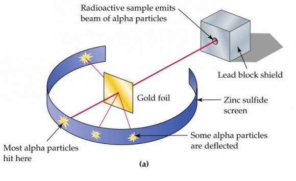
Subsequent experiments revealed a number of scientific problems with the Plum Pudding model. For starters, there was the problem of demonstrating that the atom possessed a uniform positive background charge, which came to be known as the “Thomson Problem”. Five years later, the model would be disproved by Hans Geiger and Ernest Marsden, who conducted a series of experiments using alpha particles and gold foil – aka. the “gold foil experiment.”
In this experiment, Geiger and Marsden measured the scattering pattern of the alpha particles with a fluorescent screen. If Thomson’s model were correct, the alpha particles would pass through the atomic structure of the foil unimpeded. However, they noted instead that while most shot straight through, some of them were scattered in various directions, with some going back in the direction of the source.
Diagram detailing the “gold foil experiment” conducted by Hans Geiger and Ernest Marsden. Credit: glogster.com
Geiger and Marsden concluded that the particles had encountered an electrostatic force far greater than that allowed for by Thomson’s model. Since alpha particles are just helium nuclei (which are positively charged) this implied that the positive charge in the atom was not widely dispersed, but concentrated in a tiny volume. In addition, the fact that those particles that were not deflected passed through unimpeded meant that these positive spaces were separated by vast gulfs of empty space.
By 1911, physicist Ernest Rutherford interpreted the Geiger-Marsden experiments and rejected Thomson’s model of the atom. Instead, he proposed a model where the atom consisted of mostly empty space, with all its positive charge concentrated in its center in a very tiny volume, that was surrounded by a cloud of electrons. This came to be known as the Rutherford Model of the atom.
The Bohr Model:
Subsequent experiments by Antonius Van den Broek and Niels Bohr refined the model further. While Van den Broek suggested that the atomic number of an element is very similar to its nuclear charge, the latter proposed a Solar-System-like model of the atom, where a nucleus contains the atomic number of positive charge and is surrounded by an equal number of electrons in orbital shells (aka. the Bohr Model).
In addition, Bohr’s model refined certain elements of the Rutherford model that were problematic. These included the problems arising from classical mechanics, which predicted that electrons would release electromagnetic radiation while orbiting a nucleus. Because of the loss in energy, the electron should have rapidly spiraled inwards and collapsed into the nucleus. In short, this atomic model implied that all atoms were unstable.
Diagram of an electron dropping from a higher orbital to a lower one and emitting a photon. Image Credit: Wikicommons
The model also predicted that as electrons spiraled inward, their emission would rapidly increase in frequency as the orbit got smaller and faster. However, experiments with electric discharges in the late 19th century showed that atoms only emit electromagnetic energy at certain discrete frequencies.
Bohr resolved this by proposing that electrons orbiting the nucleus in ways that were consistent with Planck’s quantum theory of radiation. In this model, electrons can occupy only certain allowed orbitals with a specific energy. Furthermore, they can only gain and lose energy by jumping from one allowed orbit to another, absorbing or emitting electromagnetic radiation in the process.
These orbits were associated with definite energies, which he referred to as energy shells or energy levels. In other words, the energy of an electron inside an atom is not continuous, but “quantized”. These levels are thus labeled with the quantum number n (n=1, 2, 3, etc.) which he claimed could be determined using the Ryberg formula – a rule formulated in 1888 by Swedish physicist Johannes Ryberg to describe the wavelengths of spectral lines of many chemical elements.
Influence of the Bohr Model:
While Bohr’s model did prove to be groundbreaking in some respects – merging Ryberg’s constant and Planck’s constant (aka. quantum theory) with the Rutherford Model – it did suffer from some flaws which later experiments would illustrate. For starters, it assumed that electrons have both a known radius and orbit, something that Werner Heisenberg would disprove a decade later with his Uncertainty Principle.
In addition, while it was useful for predicting the behavior of electrons in hydrogen atoms, Bohr’s model was not particularly useful in predicting the spectra of larger atoms. In these cases, where atoms have multiple electrons, the energy levels were not consistent with what Bohr predicted. The model also didn’t work with neutral helium atoms.
The Bohr model also could not account for the Zeeman Effect, a phenomenon noted by Dutch physicists Pieter Zeeman in 1902, where spectral lines are split into two or more in the presence of an external, static magnetic field. Because of this, several refinements were attempted with Bohr’s atomic model, but these too proved to be problematic.
In the end, this would lead to Bohr’s model being superseded by quantum theory – consistent with the work of Heisenberg and Erwin Schrodinger. Nevertheless, Bohr’s model remains useful as an instructional tool for introducing students to more modern theories – such as quantum mechanics and the valence shell atomic model.
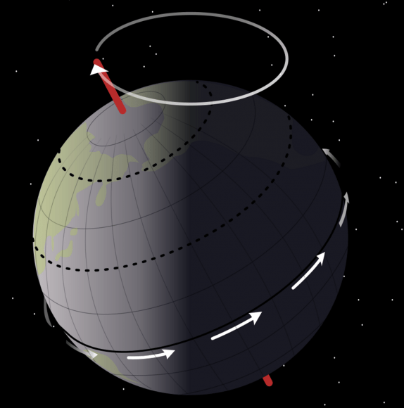
Earth's axial tilt (or obliquity) and its relation to the rotation axis and plane of orbit. Credit: Wikipedia Commons
In ancient times, the scholars, seers and magi of various cultures believed that the world took a number of forms – ranging from a ziggurat or a cube to the more popular flat disc surrounded by a sea. But thanks to the ongoing efforts of astronomers, we have come to understand that it is in fact a sphere, and one of many planets in a system that orbits the Sun.
Within the past few centuries, improvements in both scientific instruments and more comprehensive observations of the heavens have also helped astronomers to determine (with extreme accuracy) what the nature of Earth’s orbit is. In addition to knowing the precise distance from the Sun, we also know that our planet orbits the Sun with one pole constantly tilted towards it.
Earth’s Axis:
This is what is known axial tilt, where a planet’s vertical axis is tilted a certain degree towards the ecliptic of the object it orbits (in this case, the Sun). Such a tilt results in there being a difference in how much sunlight reaches a given point on the surface during the course of a year. In the case of Earth, the axis is tilted towards the ecliptic of the Sun at approximately 23.44° (or 23.439281° to be exact).
Earth’s axis points north to Polaris, the northern hemisphere’s North Star, and south to dim Sigma Octantis. Credit: Bob King
Seasonal Variations:
This tilt in Earth’s axis is what is responsible for seasonal changes during the course of the year. When the North Pole is pointed towards the Sun, the northern hemisphere experiences summer and the southern hemisphere experiences winter. When the South Pole is pointed towards the Sun, six months later, the situation is reversed.
In addition to variations in temperature, seasonal changes also result in changes to the diurnal cycle. Basically, in the summer, the day last longer and the Sun climbs higher in the sky. In winter, the days become shorter and the Sun is lower in the sky. In northern temperate latitudes, the Sun rises north of true east during the summer solstice, and sets north of true west, reversing in the winter. The Sun rises south of true east in the summer for the southern temperate zone, and sets south of true west.
The situation becomes extreme above the Arctic Circle, where there is no daylight at all for part of the year, and for up to six months at the North Pole itself (known as a “polar night”). In the southern hemisphere, the situation is reversed, with the South Pole oriented opposite the direction of the North Pole and experiencing what is known as a “midnight sun” (a day that lasts 24 hours).
The four seasons can be determined by the solstices (the point of maximum axial tilt toward or away from the Sun) and the equinoxes (when the direction of tilt and the Sun are perpendicular). In the northern hemisphere, winter solstice occurs around December 21st, summer solstice around June 21st, spring equinox around March 20th, and autumnal equinox on or about September 22nd or 23rd. In the southern hemisphere, the situation is reversed, with the summer and winter solstices exchanged and the spring and autumnal equinox dates swapped.
Changes Over Time:
The angle of the Earth’s tilt is relatively stable over long periods of time. However, Earth’s axis does undergo a slight irregular motion known as nutation – a rocking, swaying, or nodding motion (like a gyroscope) – that has a period of 18.6 years. Earth’s axis is also subject to a slight wobble (like a spinning top), which is causing its orientation to change over time.
Known as precession, this process is causing the date of the seasons to slowly change over a 25,800 year cycle. Precession is not only the reason for the difference between a sidereal year and a tropical year, it is also the reason why the seasons will eventually flip. When this happens, summer will occur in the northern hemisphere during December and winter during June.
Artist’s rendition of the Earth’s rotation and the precession of the Equinoxes. Credit: NASA
Precession, along with other orbital factors, is also the reason for what is known as “length-of-day variation”. Essentially, this is a phenomna where the dates of Earth’s perihelion and aphelion (which currently take place on Jan. 3rd and July 4th, respectively) change over time. Both of these motions are caused by the varying attraction of the Sun and the Moon on the Earth’s equatorial region.
Needless to say, Earth’s rotation and orbit around the Sun are not as simple we once though. During the Scientific Revolution, it was a huge revelation to learn that the Earth was not a fixed point in the Universe, and that the “celestial spheres” were planets like Earth. But even then, astronomers like Copernicus and Galileo still believed that the Earth’s orbit was a perfect circle, and could not imagine that its rotation was subject to imperfections.
It’s only been with time that the true nature of our planet’s inclination and movements have come to be understood. And what we know is that they lead to some serious variations over time – both in the short run (i.e. seasonal change), and in the long-run.
The eccentricity in Mars' orbit means that it is . Credit: NASA
With the Scientific Revolution, astronomers became aware of the fact that the Earth and the other planets orbit the Sun. And thanks to Copernicus, Galileo, Kepler, and Newton, the study of their orbits was refined to the point of mathematical precision. And with the subsequent discoveries of Uranus, Neptune, Pluto and the Kuiper Belt Objects, we have come to understand just how varied the orbits of the Solar Planets are.
Consider Mars, Earth’s second-closest neighbor, and a planet that is often referred to as “Earth’s Twin”. While it has many things in common with Earth, one area in which they differ greatly is in terms of their orbits. In addition to being farther from the Sun, Mars also has a much more elliptical orbit, which results in some rather interesting variations in temperature and weather patterns.
Perihelion and Aphelion:
Mars orbits the Sun at an average distance (semi-major axis) of 228 million km (141.67 million mi), or 1.524 astronomical units (over one and a half times the distance between Earth and the Sun). However, Mars also has the second most eccentric orbit of all the planets in the Solar System (0.0934), which makes it a distant second to crazy Mercury (at 0.20563).
This means that Mars’ distance from the Sun varies between perihelion (its closest point) and aphelion (its farthest point). In short, the distance between Mars and the Sun ranges during the course of a Martian year from 206,700,000 km (128.437 million mi) at perihelion and 249,200,000 km (154.8457 million mi) at aphelion – or 1.38 AU and 1.666 AU.
Speaking of a Martian year, with an average orbital speed of 24 km/s, Mars takes the equivalent of 687 Earth days to complete a single orbit around the Sun. This means that a year on Mars is equivalent to 1.88 Earth years. Adjusted for Martian days (aka. sols) – which last 24 hours, 39 minutes, and 35 seconds – that works out to a year being 668.5991 sols long (still almost twice as long).
Mars in also the midst of a long-term increase in eccentricity. Roughly 19,000 years ago, it reached a minimum of 0.079, and will peak again at an eccentricity of 0.105 (with a perihelion distance of 1.3621 AU) in about 24,000 years. In addition, the orbit was nearly circular about 1.35 million years ago, and will be again one million years from now.
Axial Tilt:
Much like Earth, Mars also has a significantly tilted axis. In fact, with an inclination of 25.19° to its orbital plane, it is very close to Earth’s own tilt of 23.439°. This means that like Earth, Mars also experiences seasonal variations in terms of temperature. On average, the surface temperature of Mars is much colder than what we experience here on Earth, but the variation is largely the same.
Mars eccentric orbit and axial tilt result in considerable seasonal variations. Credit and Copyright: Encyclopedia Britannica
All told, the average surface temperature on Mars is -46 °C (-51 °F). This ranges from a low of -143 °C (-225.4 °F), which takes place during winter at the poles; and a high of 35 °C (95 °F), which occurs during summer and midday at the equator. This means that at certain times of the year, Mars is actually warmer than certain parts of Earth.
Orbit and Seasonal Changes:
Mars’ variations in temperature and its seasonal changes are also related to changes in the planet’s orbit. Essentially, Mars’ eccentric orbit means that it travels more slowly around the Sun when it is further from it, and more quickly when it is closer (as stated in Kepler’s Three Laws of Planetary Motion).
Mars’ aphelion coincides with Spring in its northern hemisphere, which makes it the longest season on the planet – lasting roughly 7 Earth months. Summer is second longest, lasting six months, while Fall and Winter last 5.3 and just over 4 months, respectively. In the south, the length of the seasons is only slightly different.
Mars is near perihelion when it is summer in the southern hemisphere and winter in the north, and near aphelion when it is winter in the southern hemisphere and summer in the north. As a result, the seasons in the southern hemisphere are more extreme and the seasons in the northern are milder. The summer temperatures in the south can be up to 30 K (30 °C; 54 °F) warmer than the equivalent summer temperatures in the north.
Mars’ south polar ice cap, seen in April 2000 by the Mars Odyssey probe. Credit: NASA/JPL/MSSS
It also snows on Mars. In 2008, NASA’s Phoenix Landerfound water ice in the polar regions of the planet. This was an expected finding, but scientists were not prepared to observe snow falling from clouds. The snow, combined with soil chemistry experiments, led scientists to believe that the landing site had a wetter and warmer climate in the past.
And then in 2012, data obtained by the Mars Reconnaissance Orbiter revealed that carbon-dioxide snowfalls occur in the southern polar region of Mars. For decades, scientists have known that carbon-dioxide ice is a permanent part of Mars’ seasonal cycle and exists in the southern polar caps. But this was the first time that such a phenomena was detected, and it remains the only known example of carbon-dioxide snow falling anywhere in our solar system.
For starters, soil samples and orbital observation have demonstrated conclusively that roughly 3.7 billion years ago, the planet had more water on its surface than is currently in the Atlantic Ocean. Similarly, atmospheric studies conducted on the surface and from space have proven that Mars also had a viable atmosphere at that time, one which was slowly stripped away by solar wind.
Scientists were able to gauge the rate of water loss on Mars by measuring the ratio of water and HDO from today and 4.3 billion years ago. Credit: Kevin Gill
Weather Patterns:
These seasonal variations allow Mars to experience some extremes in weather. Most notably, Mars has the largest dust storms in the Solar System. These can vary from a storm over a small area to gigantic storms (thousands of km in diameter) that cover the entire planet and obscure the surface from view. They tend to occur when Mars is closest to the Sun, and have been shown to increase the global temperature.
The first mission to notice this was the Mariner 9 orbiter, which was the first spacecraft to orbit Mars in 1971, it sent pictures back to Earth of a world consumed in haze. The entire planet was covered by a dust storm so massive that only Olympus Mons, the giant Martian volcano that measures 24 km high, could be seen above the clouds. This storm lasted for a full month, and delayed Mariner 9‘s attempts to photograph the planet in detail.
And then on June 9th, 2001, the Hubble Space Telescope spotted a dust storm in the Hellas Basin on Mars. By July, the storm had died down, but then grew again to become the largest storm in 25 years. So big was the storm that amateur astronomers using small telescopes were able to see it from Earth. And the cloud raised the temperature of the frigid Martian atmosphere by a stunning 30° Celsius.
These storms tend to occur when Mars is closest to the Sun, and are the result of temperatures rising and triggering changes in the air and soil. As the soil dries, it becomes more easily picked up by air currents, which are caused by pressure changes due to increased heat. The dust storms cause temperatures to rise even further, leading to Mars’ experiencing its own greenhouse effect.
We’ve covered the full range of exotic star-type objects in the Universe. Like Pokemon Go, we’ve collected them all. Okay fine, I’m still looking for a Tauros, and so I’ll continue to wander the streets, like a zombie staring at his phone.
Now, according to my attorney, I’ve fulfilled the requirements for shamelessly jumping on a viral bandwagon by mentioning Pokemon Go and loosely connecting it to whatever completely unrelated topic I was working on.
Any further Pokemon Go references would just be shameless attempts to coopt traffic to my channel, and I’m better than that.
It was pretty convenient, though, and it was easy enough to edit out the references to Quark on Deep Space 9 and replace them with Pokemon Go. Of course, there is a new Star Trek movie out, so maybe I miscalculated.
Anyway, now that we got that out of the way. Back to rare and exotic stellar objects.
The white dwarf G29-38. Credit: NASA
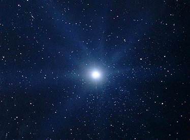
There are the white dwarfs, the remnants of stars like our Sun which have passed through the main sequence phase, and now they’re cooling down.
There are the neutron stars and pulsars formed in a moment when stars much more massive than our Sun die in a supernova explosion. Their gravity and density is so great that all the protons and electrons from all the atoms are mashed together. A single teaspoon of neutron star weighs 10 million tons.
And there are the black holes. These form from even more massive supernova explosions, and the gravity and density is so strong they overcome the forces holding atoms themselves together.
White dwarfs, neutron stars and black holes. These were all theorized by physicists, and have all been discovered by observational astronomers. We know they’re out there.
Is that it? Is that all the exotic forms that stars can take? That we know of, yes, however, there are a few even more exotic objects which are still just theoretical. These are the quark stars. But what are they?
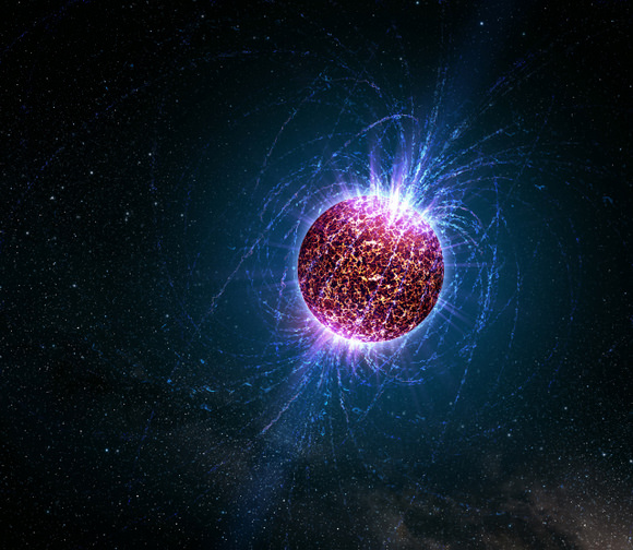
Artist concept of a neutron star. Credit: NASA
Let’s go back to the concept of a neutron star. According to the theories, neutron stars have such intense gravity they crush protons and electrons together into neutrons. The whole star is made of neutrons, inside and out. If you add more mass to the neutron star, you cross this line where it’s too much mass to hold even the neutrons together, and the whole thing collapses into a black hole.
A star like our Sun has layers. The outer convective zone, then the radiative zone, and then the core down in the center, where all the fusion takes place.
Could a neutron star have layers? What’s at the core of the neutron star, compared to the surface?
The idea is that a quark star is an intermediate stage in between neutron stars and black holes. It has too much mass at its core for the neutrons to hold their atomness. But not enough to fully collapse into a black hole.
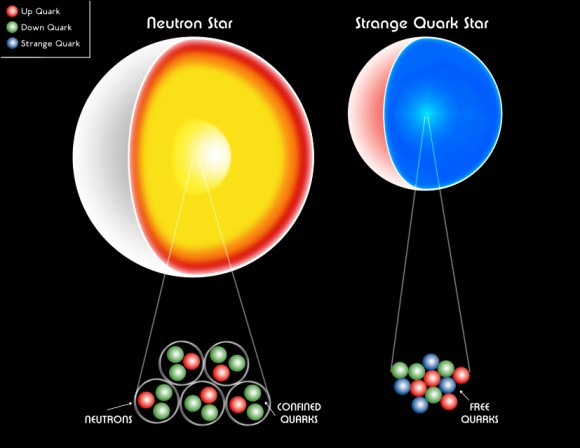
The difference between a neutron star and a quark star. Credit: Chandra
In these objects, the underlying quarks that form the neutrons are further compressed. “Up” and “down” quarks are squeezed together into “strange” quarks. Since it’s made up of “strange” quarks, physicists call this “strange matter”. Neutron stars are plenty strange, so don’t give it any additional emotional weight just because it’s called strange matter. If they happened to merge into “charm” quarks, then it would be called “charm matter”, and I’d be making Alyssa Milano references.
And like I said, these are still theoretical, but there is some evidence that they might be out there. Astronomers have discovered a class of supernova that give off about 100 times the energy of a regular supernova explosion. Although they could just be mega supernovae, there’s another intriguing possibility.
They might be heavy, unstable neutron stars that exploded a second time, perhaps feeding from a binary companion star. As they hit some limit, they converting from a regular neutron star to one made of strange quarks.
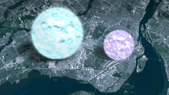
But if quark stars are real, they’re very small. While a regular neutron star is 25 km across, a quark star would only be 16 km across, and this is right at the edge of becoming a black hole.
A neutron star (~25km across) next to a quark star (~16km across). Original Image Credit: NASA’s Goddard Space Flight Center
If quark stars do exist, they probably don’t last long. It’s an intermediate step between a neutron star, and the final black hole configuration. A last gasp of a star as its event horizon forms.
It’s intriguing to think there are other exotic objects out there, formed as matter is compressed into tighter and tighter configurations, as the different limits of physics are reached and then crossed. Astronomers will keep searching for quark stars, and I’ll let you know if they find them.
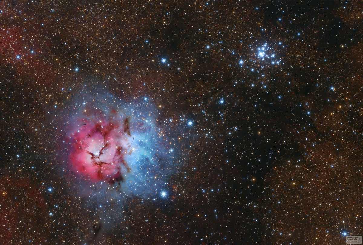
The Triffid Nebula (on the left), with M21 open star cluster to the right. Credit and Copyright: NASA/Lorand Fenyes
Welcome back to Messier Monday! In our ongoing tribute to the great Tammy Plotner, we take a look at the Trifid Nebula (aka. Messier 20). Enjoy!
Back in the 18th century, famed French astronomer Charles Messier noted the presence of several “nebulous objects” in the night sky. Having originally mistaken them for comets, he began compiling a list of these objects so that others wouldn’t make the same mistake. Consisting of 100 objects, the Messier Catalog would come to be viewed by posterity as a major milestone in the study of Deep Space Objects.
One of these objects is the Trifid Nebula (aka. Messier 20, NGC 6514), a star-forming region of ionized gas located in the Scutum spiral arm of the Milky Way, in the direction of the southern Sagittarius constellation. A bright object that is a favorite amongst amateur astronomers, this object is so-named because it is a combination open star cluster, emissions nebula, reflection nebula, and a dark nebula that looks like it consists of three lobes.
Description:
Almost everyone who is familiar with space images has likely seen a beautiful color image of this emission and reflection nebula. However, when looking at M20 through a telescope, what you will see will be less colorful. Why? When it comes to photographs, exposure times and wavelengths cause different colors to become visible.
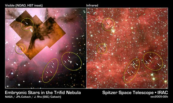
Composite image comparing visible-light views from Hubble of the Trifid Nebula with an infrared view from NASA’s Spitzer Space Telescope of the glowing Trifid Nebula. Credit: NASA/JPL-Caltech/J. Rho (SSC/Caltech)
Photographically, the red emission nebula contained within Messier 20 has a bright blue star cluster in it central portion. It glows red because the ultraviolet light of the stars ionizes the hydrogen gas, which then recombines and emits the characteristic red hydrogen-alpha light captured on film. Further away, the radiation from these hot, young stars becomes too weak to ionize the hydrogen. Now the gas and dust glows blue by reflection!
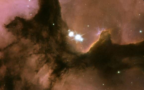
No matter how it is observed, the Trifid – or “three lobed” – nebula has a distinctive set of dark dust lanes which divide it. These also have a classification of their own, and were cataloged by E.E. Barnard as a dark nebula – Barnard 85 (B 85). In 1999 the Hubble Space Telescope took a look deep into the Trifid nebula at some of its star forming regions (see below).
What it found was a stellar jet poking its way into the cloud, like a fabulous twisted antenna. Inside the exhaust column is a new star waiting to be born, yet sometime over the next 10,000 years the central massive star will probably erode away all of its material before it can fully form. Nearby, a stalk stands waiting.
Close up on the interior of the Trifid Nebula, showing the star forming region and a stellar jet. Credit: NASA/HST
Like the jet, it is also a stellar nursery – one with an EGG (evaporating gaseous globule) at its tip – a condensed cloud of gas able to survive so far. As Jeff Hester of the Department of Physics & Astronomy explained:
“If our interpretation is correct, the microjet may be the last gasp from a star that was cut off from its supply lines 100,000 years ago. The vast majority of stars like our sun form not in isolation, but in the neighborhood of massive, powerful stars. HST observations of the Trifid Nebula provide a window on the nature of star formation in the vicinity of massive stars, as well as a spectacular snapshot of the “ecology” from which stars like our sun emerge.”
“We report the discovery of a new candidate barrel-shaped supernova remnant (SNR) lying adjacent to M20 and two shell-type features to the north and east of SNR W28. Future observations should clarify whether the nonthermal shell fragment is either part of W20 or yet another previously unidentified shell-type SNR.”
The Trifid nebula (M20, NGC NGC 6514) in pseudocolor. Image taken with the Palomar 1.5-m telescope. Credit: Jeff Hester (Arizona State University)/Palomar telescope
History of Observation:
Charles Messier discovered this object on June 5th, 1764. As he recorded of the object in his notes:
“In the same night I have determined the position of two clusters of stars which are close to each other, a bit above the Ecliptic, between the bow of Sagittarius and the right foot of Ophiuchus: the known star closest to these two clusters is the 11th of the constellation Sagittarius, of seventh magnitude, after the catalog of Flamsteed: the stars of these clusters are, from the eighth to the ninth magnitude, environed with nebulosities. I have determined their positions. The right ascension of the first cluster, 267d 4′ 5″, its declination 22d 59′ 10″ south. The right ascension of the second, 267d 31′ 35″; its declination, 22d 31′ 25″ south.”
While Messier did separate the two star clusters, he did not note so many different portions to the nebula – but, he did note nebulosity. In this circumstance, we cannot fault him. His purpose was to locate comets, after all; and the reason for the catalog was to list objects that were not. In later years, it would be Sir William Herschel who would take a closer look at Messier 20 and discover much more. As he wrote of the nebula:
“If it was supposed that double nebulae at some distance from each other would frequently be seen, it will now on the contrary be admitted that an expectation of finding a great number of attracting centers in a nebulosity of no great extent is not so probable; and accordingly observation has shewn that greater combinations of nebular than those of the foregoing article are less frequently to be seen. The following list however contains 20 treble, 5 quadruple, and 1 sextuple nebulae of this sort. Among the treble nebulae there is one, namely H V.10 [M20], of which the nebulosity is not yet separated. Three nebulae seem to join faintly together, forming a kind of triangle; the middle of which is less nebulous, or perhaps free of nebulosity; in the middle of the triangle is a double star of the 2nd or 3rd class; more faint nebulosities are following.”
A close detail of the Trifid Nebula, showing a “Pillar” region. Credit: NASA/Jeff Hester (Arizona State University).
While William went on to catalog four separate areas in his books, it was his son John to whom we owe the famous name that we know it by today. “A most remarkable object. Very large; trifid, three nebulae with a vacuity in the midst, in which is centrally situated the double star Sh 379, the nebula is 7′ in extent. A most remarkable object.”
Just remember when you observe that sky conditions are everything and that not even a large telescope can make it appear if the sky isn’t right. Even Admiral Smyth has his share of troubles spotting it. Said he of the Trifid Nebula:
“I lowered the telescope a couple of degrees, and gazed for the curious trifid nebula, 41 H. IV [H IV.41]; but though I could make out the delicate triple star in the centre of its opening, the nebulous matter resisted the light of my telescope, so that its presence was only indicated by a peculiar glow. Pretty closely preceding this is No. 20 M., an elegant cruciform group of stars, discovered in 1764, which he considered to be surrounded with nebulosity.”
Locating Messier 20:
Once you have become familiar with the Sagittarius region, finding Messier 20 is easy, since it is located just 2 degrees northwest of Messier 8 – the “Lagoon” Nebula. However, at magnitude 9, it isn’t an easy to spot with small binoculars, and not always easy for a small telescope either. Because we often see it depicted in pictures as bright and beautiful, we simply assume M20 will jump out of the sky; but you’ll find that its a lot fainter and more elusive than you might think.
The Sagittarius constellation. Credit: iau.org
If you are a beginner to astronomy, try starting at the teapot’s tip star (Lambda), “Al Nasl”, and starhopping in the finderscope northwest to the Lagoon. While the nebulosity might not show in your finder, the optical double star 7 Sagittari, will. From there you will spot a bright cluster of stars two degrees due north. These are the stars embedded withing the Trifid and the small, compressed area of stars to its northeast is the open star cluster of Messier 21.
Center your finderscope on the north and south oriented pair of stars and observe. Remember that you will need a moonless night and that sky conditions will need to be right to see the dark dustlanes! And here are the quick facts about M20, for your convenience:
Object Name: Messier 20 Alternative Designations: M20, NGC 6514, Trifid Nebula Object Type: Emission Nebula and Reflection Nebula with Open Star Cluster Constellation: Sagittarius Right Ascension: 18 : 02.6 (h:m) Declination: -23 : 02 (deg:m) Distance: 5.2 (kly) Visual Brightness: 9.0 (mag) Apparent Dimension: 28.0 (arc min)


![The Trifid nebula (M20, NGC NGC 6514) in pseudocolor. Image taken with the Palomar 1.5-m telescope. The field of view is 16’ ´ 16’. Red shows [S II] ll 6717+6731. Green shows Ha l 6563. Blue shows [O III] l 5007. The WFPC2 field of view is indicated. Image: Jeff Hester (Arizona State University), Palomar telescope.](https://www.universetoday.com/wp-content/uploads/2009/06/Trifid-Nebula-M20-e1469471610624-580x515.jpg)