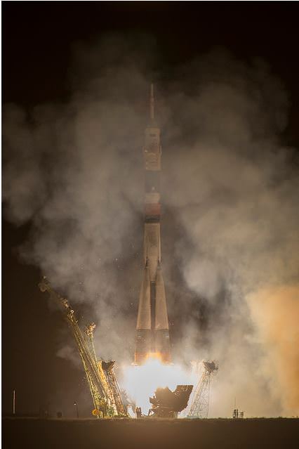
Catch the Moon pairing with Mercury & Venus Tonight

Looking west at sunset from latitude 30 degrees north. The ecliptic and Mercury's orbit along with a 10 degree field of view outlined for reference. All graphics created by the author using Starry Night).

If you’ve never seen Mercury, this week is a great time to try.

Over the past few weeks, observers worldwide have been following the outstanding tight triple conjunction of Mercury, Venus and Jupiter low to the west at dusk.

Jupiter has exited the evening sky, headed for conjunction with the Sun on June 19th. I caught what was probably our last glimpse of Jupiter for the season clinging to the murky horizon through binoculars just last week. If you’re “Jonesin’ for Jove,” you can follow its progress this week through superior conjunction as it transits the Solar Heliospheric Observatory’s LASCO C3 camera.

This leaves the two innermost worlds of our fair solar system visible low to the west at dusk. And tonight, they’re joined by a very slender waxing crescent Moon, just over two days after New phase.

The Moon, Venus and Mercury as seen from 30 degrees north tonight at 9PM EDT.

The evening of June 10th finds a 4% illuminated Moon passing just over 5 degrees (about 10 Full Moon diameters) south of Venus and Mercury. Venus will be the first to appear as the sky darkens, shining at magnitude -3.9 and Mercury will shine about 40 times fainter above it at magnitude +0.3.

Ashen light, also known as Earthshine will also be apparent on the darkened limb of the Moon. Another old-time term for this phenomenon is “the Old Moon in the New Moon’s Arms.” Ashen light is caused by sunlight being reflected off of the Earth and illuminating the nighttime Earthward facing portion of the Moon. Just how prominent this effect appears can vary depending on the total amount of cloud cover on the Earth’s Moonward facing side.

....and the orientation of the Moon, Mercury and Venus on the night of June 12th and ~9PM EDT.
….and the orientation of the Moon, Mercury and Venus on the night of June 12th and ~9PM EDT.

This week sets the stage for the best dusk apparition of Mercury for northern hemisphere viewers in 2013. Orbiting the Sun every 88 Earth days, we see Mercury either favorably placed east of the Sun in the dusk sky or west of the Sun in the dawn sky roughly six times a year. Mercury’s orbit is markedly elliptical, and thus not all apparitions are created the same. An elongation near perihelion, when Mercury is 46 million kilometers from the Sun, can mean its only 17.9 degrees away from the Sun as viewed from the Earth. An elongation near aphelion, 69.8 million kilometers distant, has a maximum angular separation of 27.8 degrees.

This week’s greatest elongation of 24.3 degrees occurs on June 12th. It’s not the most extreme value for 2013, but does have another factor going for it; the angle of the ecliptic. As we approach the solstice of June 21st, the plane of the solar system as traced out by the orbit of the Earth is at a favorable angle relative to the horizon. Thus, an observer from 35 degrees north latitude sees Mercury 18.4 degrees above the horizon at sunset, while an observer at a similar latitude in the southern hemisphere only sees it slightly lower at 16.9 degrees.

Venus and the Moon make great guides to locate Mercury over the next few nights. It’s said that Copernicus himself never saw Mercury with his own eyes, though this oft repeated tale is probably apocryphal.

We also get a shot at a skewed “emoticon conjunction” tonight, not quite a “smiley face” (: as occurred between Jupiter, Venus and the Moon in 2008, but more of a “? :” Stick around until February 13th, 2056 and you’ll see a much tighter version of the same thing! A time exposure of a pass of the International Space Station placed near Mercury and Venus could result in a planetary “meh” conjunction akin to a “/:” Hey, just throwing that obscure challenge out there. Sure, there’s no scientific value to such alignments, except as testimony that the universe may just have a skewed sense of humor…

Through the telescope, Venus currently shows a 10” diameter gibbous phase, while Mercury is only slightly smaller at 8” and is just under half illuminated. No detail can be discerned on either world, as a backyard telescope will give you the same blank view of both worlds that vexed astronomers for centuries. These worlds had to await the dawn of the space age to give up their secrets. NASA’s MESSENGER spacecraft entered a permanent orbit around Mercury in 2011, and continues to return some outstanding science.

Both planets are catching up to us from the far side of their orbits. Mercury will pass within 2 degrees of Venus on June 20th, making for a fine wide field view in binoculars.

And now for the wow factor of what you’re seeing tonight. The Moon just passed apogee on June 9th and is currently about 416,500 kilometers or just over one light second distant. Mercury meanwhile, is 0.86 astronomical units (A.U.), or almost 133 million kilometers, or about 7 light minutes away. Finally, Venus is currently farther away from the Earth than the Sun at 1.59 A.U.s, or about 13.7 light minutes distant.

All this makes for a great show in the dusk skies this week. And yes, lunar apogee just after New sets us up for the closest Full Moon of 2013 (aka the internet sensation known as the “Super Moon”) on June 23rd. More to come on that soon!


Observing Alert: Rare Meteor Shower May ‘Outburst’ on June 11

The rare and rarely heard of meteor shower called the Gamma Delphinids will appear to radiate from the constellation Delphinus (del-FINE-us) the Dolphin high in the southern sky shortly before dawn tomorrow morning June 11. This map shows the sky facing south at 3:30 a.m. local time. Delphinus is near the bottom of the bright 3-star figure the Summer Triangle. Stellarium

Back on June 11, 1930 three members of the American Meteor Society (AMS) in Maryland saw a half-hour-long bright outburst of meteors from the little constellation Delphinus the Dolphin. No one had predicted the shower, but it came out of nowhere and hasn’t been seen since. Attempts to catch a repeat performance in subsequent years met with no success.

That may change tomorrow morning, June 11, 2013. Peter Jenniskins, research scientist with the SETI Institute and NASA Ames Research Center, has examined dust outbursts from long-period comets and suggests the Gamma Delphinids may return for a brief moment of splendor, as Earth passes through this stream of cometary debris not seen since 1930.

Bright meteors photographed in Ohio during the Eta Aquarid meteor shower in 2012. The Gamma Delphinids may send similar bright meteors our way tomorrow morning. Credit: John Chumack

The expected time of maximum activity is 4:30 a.m. Eastern Daylight Time, 3:30 a.m. Central, 2:30 a.m. Mountain and 1:30 a.m. Pacific. These times are ideal for the Americas where Delphinus is high in southern sky at the peak time. Robert Lunsford of the AMS recommends starting your Gamma Delphinid vigil 2 hours ahead of time in case the shower’s early. If these meteors really do happen, you’ll see them anywhere in the sky, but they’ll all trace back to a point near the star Gamma Delphini in the dolphin’s nose.

The map above shows the worldwide possible visibility for the gamma Delphinid shower. Visibility will be best in the bright green areas, which have the highest radiant elevation. Unshaded areas on the map will not have a view of the shower. Credit: Geert Barentsen, International Meteor Organization

No one knows how strong the shower might be or even the duration though it’s likely to be brief. Time estimate range from one hour to 15 minutes. Lunsford expects bright meteors to appear a minute or two apart.  If you’re game, split the difference and set up in a comfy lawn chair facing south an hour before the expected maximum. Should you see any of these rare dolphin tears, consider e-mailing a report to: [email protected]

Tonight June 10-11 from 10 p.m. – 2 a.m. CDT, Dr. Bill Cooke of NASA’s Meteoroid Environment Office will take your questions via live web chat. He’ll offer viewing tips about the shower and include a live Ustream telescope view of the skies over Huntsville, Ala.

If you shoot video or images and want to help improve our understanding of this elusive meteor shower, you can upload them to the Office’s Flickr group and also to Universe Today’s Flickr group. We’ll post images if this meteor shower proves to show up!

Kapow! Keck Confirms Puzzling Element of Big Bang Theory

Illustration of the Big Bang Theory
The Big Bang Theory: A history of the Universe starting from a singularity and expanding ever since. Credit: grandunificationtheory.com

Observations of the kaboom that built our universe — known as the Big Bang — is better matching up with theory thanks to new work released from one of the twin 33-foot (10-meter) W.M. Keck Observatory telescopes in Hawaii.

For two decades, scientists were puzzled at a lithium isotope discrepancy observed in the oldest stars in our universe, which formed close to the Big Bang’s occurrence about 13.8 billion years ago. Li-6 was about 200 times more than predicted, and there was 3-5 times less Li-7 — if you go by astronomical theory of the Big Bang.

The fresh work, however, showed that these past observations came up with the strange numbers due to lower-quality data that, in its simplifications, created more lithium isotopes detections than are actually present. Keck’s observations found no discrepancy.

Artist's conception of a metal-poor star. Astronomers modelled a portion of its surface to figure out its abundance of lithium-6, an element that was previously in discrepancy between Big Bang theory and observations of old stars. Credit: Karin Lind, Davide De Martin.
Artist’s conception of a metal-poor star. Astronomers modelled a portion of its surface to figure out its abundance of lithium-6, an element that was previously in discrepancy between Big Bang theory and observations of old stars. Credit: Karin Lind, Davide De Martin.

“Understanding the birth of our universe is pivotal for the understanding of the later formation of all its constituents, ourselves included,” stated lead researcher Karin Lind, who was with the Max Planck Institute for Astrophysics in Munich when the work was performed.

“The Big Bang model sets the initial conditions for structure formation and explains our presence in an expanding universe dominated by dark matter and energy,” added Lind, who is now with the University of Cambridge.

To be sure, it is difficult to measure lithium-6 and lithium-7 because their spectroscopic “signatures” are pretty hard to see. It takes a large telescope to be able to do it. Also, modelling the data can lead to accidental detections of lithium because some of the processes within these old stars appear similar to a lithium signature.

Keck used a high-resolution spectrometer to get the images and gazed at each star for several hours to ensure astronomers got all the photons it needed to do analysis. Modelling the data took several more weeks of work on a supercomputer.

The research appeared in the June 2013 edition of Astronomy & Astrophysics. You can check out the entire paper here.

Source: Keck Observatory

Astronomers Refine Distances to our Closest Spiral-Galaxy Neighbors

M31 and M33 are two of the nearest spiral galaxies, and can form the basis for determining distances to more remote spiral galaxies and constraining the expansion rate of the Universe (the Hubble constant).  Hence the relevance and importance of several new studies that employed near-infrared data to establish solid distances for M31 (Andromeda) and M33 (Triangulum) (e.g., Gieren et al. 2013), and aimed to reduce existing uncertainties tied to the fundamental parameters for those galaxies.  Indeed, reliable distances for M31 and M33 are particularly important in light of the new Hubble constant estimate from the Planck satellite, which is offset relative to certain other results, and that difference hinders efforts to ascertain the nature of dark energy (the mysterious force theorized as causing the Universe’s accelerated expansion).

Gieren et al. remarked that, “a number of new distance determinations to M33 … span a surprisingly large interval … which is a cause of serious concern. As the second-nearest spiral galaxy, an accurate determination of [M33’s] distance is a crucial step in the process of building the cosmic distance ladder.”  Concerning M31, Riess et al. 2012 likewise remarked that “M31, the nearest analogue of the Milky Way Galaxy, has long provided important clues to understanding the scale of the Universe.

 The new Gieren and Riess et al. distances are based on near-infrared observations, which are pertinent because radiation from that part of the electromagnetic spectrum is less sensitive than optical data to absorption by dust located along our sight-line (see the figure below).  Properly accounting for the impact of dust is a principal problem in cosmic distance scale work, since it causes targets to appear dimmer.  “different assumptions about [dust obscuration] are a prime source for the discrepancies among the various distance determinations for M33.” noted Gieren et al., and the same is true for the distance to M31 (see Riess et al.).

Optical and near-infrared images highlight how dust obscures light emitted from a target along the line-of-sight.  The near-infrared observations are less sensitive to that obscuration (image credit: Alves et al. 2001).
Optical and near-infrared images highlight how dust obscures light emitted from targets along the sight-line, and that the level of obscuration is wavelength dependent. New distances established for M31 and M33 are based on near-infrared observations, which are less sensitive to that obscuration (image credit: Alves et al. 2001).

The Gieren and Riess et al. distances to M33 and M31, respectively, were inferred from observations of Cepheids.   Cepheids are a class of variable stars that exhibit periodic brightness variations (they pulsate radially).  Cepheids can be used as distance indicators because their pulsation period and mean luminosity are correlated.  That relationship was discovered by Henrietta Leavitt in the early 1900s.  A pseudo period-luminosity relation derived for M31 Cepheids is presented below.

Gieren et al. observed 26 Cepheids in M33 and established a distance of ~2,740,000 lightyears.  The team added that, “As the first modern near-infrared Cepheid study [of] M33 since … some 30 years … we consider this work as long overdue …”  Astronomers often cite distances to objects in lightyears, which defines the time required for light emitted from the source to reach the observer. Despite the (finite) speed of light being 300,000,000 m/s, the rays must traverse “astronomical” distances.   Gazing into space affords one the unique opportunity to peer back in time.

A relation exists between a Cepheid's a periodic brightness variations and its luminosity.  Astronomers use that relation, which was discovered in the early 1900s by Henrietta Leavitt, to establish distances to galaxies.  In the above figure the horizontal axis features the pulsation period, and the vertical axis a proxy  for luminosity (image credit: Fig 2 in Riess et al., 2013 arXiv/ApJ).
A relation exists between a Cepheid’s periodic brightness variations and its mean luminosity. Astronomers use that trend, which was discovered in the early 1900s by Henrietta Leavitt, to establish distances to galaxies hosting Cepheids. In the above figure the horizontal axis features the pulsation period, and the vertical axis defines a proxy for luminosity (image credit: Fig 2 from Riess et al., arXiv/ApJ).

The distances to M33 shown below convey seminal points in the evolution of humanity’s knowledge.  The scatter near the 1920s stems partly from a debate concerning whether the Milky Way and the Universe are synonymous.  In other words, do galaxies exist beyond the Milky Way?  The topic is immortalized in the famed great debate (1920) featuring H. Shapley and H. Curtis (the latter argued for an extragalactic scale).  The offset between the pre-1930 and post-1980 data result in part from a nearly two-fold increase in the cosmic distance scale recognized circa 1950 (see also Feast 2000).   Also evident is the scatter associated with the post-1980 distances, which merely reinforces the importance of the new high-precision distance estimates.

Riess et al. obtained data for some 70 Cepheids and determined a distance for M31 of ~2,450,000 lightyears.  The latter is corroborated by a new study by Contreras Ramos et al. 2013 (d~2,540,000 ly), whose distance estimate relied on data for stars in a M31 globular cluster.

A subset of the distances estimated for M33, as compiled from estimates featured in the NASA/IPAC Extragalactic Database (Steer & Madore). On the vertical axis is the distance to the galaxy in units of lightyears, and  the year is cited on the horizontal axis.  The red arrow and black datum indicate the new near-infrared based distance from Gieren et al. 2013 (image credit: DM).
A subset of the distances deduced for M33, as compiled from estimates featured in the NASA/IPAC Extragalactic Database (Steer & Madore). On the vertical axis is the distance to the galaxy in units of lightyears, and the year is cited on the horizontal axis.  The red arrow and black datum indicate the new near-infrared based distance from Gieren et al. (image credit: DM).

Top-class instruments and telescopes are needed to obtain reliable measurements of stars in galaxies nearly 3,000,000 million lightyears away.  Gieren et al. utilized the 8.2-m Very Large Telescope (Yepun) instrument shown below, while Riess and Contreras Ramos et al. analyzed observations from the Hubble Space Telescope.  Riess et al. acquired images of M31 via the new Wide-field Camera 3, which replaced the Wide-field and Planetary Camera 2 (“The Camera That Saved Hubble“) during the famed 2009 servicing mission.

The new results mark the culmination of a century’s worth of effort aimed at securing precise distances for our Galaxy’s local spiral kin (M31 and M33).  However, the offset between the Planck and certain Cepheid/SN-based determinations of the Hubble constant demands that research continue in order to identify uncertainties associated with the methods.

Gieren et al. used the 8.2-m Very Large Telescope (Yepun) to image M33, and deduce the distance to that galaxy (image credit: ESO).
Gieren et al. used the 8.2-m Very Large Telescope (Yepun) to image stars in M33, and deduce the distance to that galaxy (image credit: G. Hüdepohl/ESO).

The Gieren et al. findings have been accepted for publication in the Astrophysical Journal (ApJ), and a preprint is available on arXiv.   Both the Riess and Contreras Ramos et al. studies are likewise published in ApJ.  The interested reader desiring additional information on the cosmic distance scale and Cepheids will find the following resources pertinent: the AAVSO’s article on Delta Cephei (the namesake for the class of Cepheid variables), Freedman & Madore (2010)Tammann & Reindl 2012, Fernie 1969, the NASA/IPAC Extragalactic Database, G. Johnson’s Miss Leavitt’s Stars: The Untold Story of the Woman Who Discovered How to Measure the Universe, D. Fernie’s Setting Sail for the Universe: Astronomers and their Discoveries, Nick Allen’s The Cepheid Distance Scale: A History, D. Turner’s Classical Cepheids After 228 Years of Study, J. Percy’s Understanding Variable Stars.

Carnival of Space #305

This week’s Carnival of Space is hosted by Peter Lake at the AartScope blog.

Click here to read Carnival of Space #305.

And if you’re interested in looking back, here’s an archive to all the past Carnivals of Space. If you’ve got a space-related blog, you should really join the carnival. Just email an entry to [email protected], and the next host will link to it. It will help get awareness out there about your writing, help you meet others in the space community – and community is what blogging is all about. And if you really want to help out, sign up to be a host. Send an email to the above address.

Amazing Astrophoto: The North American Nebula by Mick Hyde

Here’s a truly gorgeous image by astrophotographer Mick Hyde, a mosaic of NGC 7000 (the North American nebula) and the Pelican nebula (IC 5070).

The structure on the upper left side is the North American nebula, with the darkest lobe of dust near the center forming the “Gulf of Mexico.” The star-forming region is located approximately 1,600 light years away in the constellation of Cygnus the Swan.

On the upper right is another celestial water bird, the Pelican nebula, a bright curve of ionized gas suggesting the shape of a pelican’s head and neck.

Check out a wider view of this region here, and see this and more of Mick’s work on his Flickr page here.

Image © Mick Hyde. Used with permission.

10 Years & Top 10 Discoveries from Marvelous Mars Express

Mars Express over water-ice crater. ESA Celebrates 10 Years since the launch of Mars Express. This artists concept shows Mars Express set against a 35 km-wide crater in the Vastitas Borealis region of Mars at approximately 70.5°N / 103°E. The crater contains a permanent patch of water-ice that likely sits upon a dune field – some of the dunes are exposed towards the top left in this image. Copyright ESA/DLR/FU-Berlin-G.Neukum

This week marks the 10th anniversary since the launch of the European Space Agencies’ (ESA) Mars Express orbiter from the Baikonur Cosmodrome in Russia on June 2, 2003 and a decade of ground breaking science discoveries at the Red Planet.

2003 was a great year for Mars exploration as it also saw the dual liftoffs of NASA’s now legendary rovers Spirit & Opportunity from Cape Canaveral in Florida.

The immense quantity and quality of science data returned from Mars Express -simultaneously with Spirit and Opportunity – has completely transformed our understanding of the history and evolution of the Red Planet.

All three spacecraft have functioned far beyond their original design lifetime.

Earth’s exploration fleet of orbiters, landers and rovers have fed insights to each other that vastly multiplied the science output compared to working solo during thousands and thousands of bonus Sols at Mars.

Inside a central pit crater.  Perspective view of a 50 km diameter crater in Thaumasia Planum. The image was made by combining data from the High-Resolution Stereo Camera on ESA’s Mars Express with digital terrain models. The image was taken on 4 January 2013, during orbit 11467, and shows a close up view of the central ‘pit’ of this crater, which likely formed by a subsurface explosion as the heat from the impact event rapidly vapourised water or ice lying below the surface. Copyright ESA/DLR/FU-Berlin-G.Neukum
Inside a central pit crater. Perspective view of a 50 km diameter crater in Thaumasia Planum. The image was made by combining data from the High-Resolution Stereo Camera on ESA’s Mars Express with digital terrain models. The image was taken on 4 January 2013, during orbit 11467, and shows a close up view of the central ‘pit’ of this crater, which likely formed by a subsurface explosion as the heat from the impact event rapidly vapourised water or ice lying below the surface. Copyright ESA/DLR/FU-Berlin-G.Neukum

Mars Express derived its name from an innovative new way of working in planetary space science that sped up the development time and cut costs in the complex interactive relationships between the industrial partners, space agencies and scientists.

Indeed the lessons learned from building and operating Mars Express spawned a sister ship, Venus Express that also still operates in Venusian orbit.

Mars Express (MEX) achieved orbit in December 2003.

MEX began science operations in early 2004 with an array of seven instruments designed to study all aspects of the Red Planet, including its atmosphere and climate, and the mineralogy and geology of the surface and subsurface with high resolution cameras, spectrometers and radar.

The mission has been granted 5 mission extensions that will carry it to at least 2014.

The mission has been wildly successful except for the piggybacked lander known as Beagle 2, which was British built.

Beagle 2
Beagle 2
The ambitious British lander was released from the mothership on December 19, 2003, six days before MEX braked into orbit around Mars. Unfortunately the Beagle 2 was never heard from again as it plummeted to the surface and likely crashed.

The high resolution camera (HRSC) has transmitted thousands of dramatic 3D images all over Mars ranging from immense volcanoes, steep-walled canyons, dry river valleys, ancient impact craters of all sizes and shapes and the ever-changing polar ice caps.

It carried the first ever radar sounder (MARSIS) to orbit another planet and has discovered vast caches of subsurface water ice.

MEX also played a significant role as a data relay satellite for transmissions during the landings of NASA’s Phoenix lander and Curiosity rover. It also occasionally relays measurements from Spirit & Opportunity to NASA.

Arima twins topography. This colour-coded overhead view is based on an ESA Mars Express High-Resolution Stereo Camera digital terrain model of the Thaumasia Planum region on Mars at approximately 17°S / 296°E. The image was taken during orbit 11467 on 4 January 2013. The colour coding reveals the relative depth of the craters, in particular the depths of their central pits, with the left-hand crater penetrating deeper than the right (Arima crater).  Copyright: ESA/DLR/FU-Berlin-G.Neukum
Arima twins topography. This colour-coded overhead view is based on an ESA Mars Express High-Resolution Stereo Camera digital terrain model of the Thaumasia Planum region on Mars at approximately 17°S / 296°E. The image was taken during orbit 11467 on 4 January 2013. The colour coding reveals the relative depth of the craters, in particular the depths of their central pits, with the left-hand crater penetrating deeper than the right (Arima crater). Copyright: ESA/DLR/FU-Berlin-G.Neukum

Here is a list of the Top 10 Discoveries from Mars Express from 2003 to 2013:

Mars Express mineralogy maps. This series of five maps shows near-global coverage of key minerals that help plot the history of Mars. The map of hydrated minerals indicates individual sites where a range of minerals that form only in the presence of water were detected. The maps of olivine and pyroxene tell the story of volcanism and the evolution of the planet’s interior. Ferric oxides, a mineral phase of iron, are present everywhere on the planet: within the bulk crust, lava outflows and the dust oxidised by chemical reactions with the martian atmosphere, causing the surface to ‘rust’ slowly over billions of years, giving Mars its distinctive red hue. Copyright:  ESA/CNES/CNRS/IAS/Université Paris-Sud, Orsay; NASA/JPL/JHUAPL; Background images: NASA MOLA
Mars Express mineralogy maps. This series of five maps shows near-global coverage of key minerals that help plot the history of Mars. The map of hydrated minerals indicates individual sites where a range of minerals that form only in the presence of water were detected. The maps of olivine and pyroxene tell the story of volcanism and the evolution of the planet’s interior. Ferric oxides, a mineral phase of iron, are present everywhere on the planet: within the bulk crust, lava outflows and the dust oxidised by chemical reactions with the martian atmosphere, causing the surface to ‘rust’ slowly over billions of years, giving Mars its distinctive red hue. Copyright: ESA/CNES/CNRS/IAS/Université Paris-Sud, Orsay; NASA/JPL/JHUAPL; Background images: NASA MOLA
#1. First detection of hydrated minerals in the form of phyllosilicates and hydrated sulfates – evidence of long periods of flowing liquid water from the OMEGA visible and infrared spectrometer provided confirmation that Mars was once much wetter than it is today and may have been favorable for life to evolve.

#2. Possible detection of methane in the atmosphere from the Planetary Fourier Spectrometer (PFS) which could originate from biological or geological activity.

#3. Identification of recent glacial landforms via images from the High Resolution Stereo Camera (HRSC) are stem from viscous flow features composed of ice-rich material derived from adjacent highlands.

#4. Probing the polar regions. OMEGA and MARSIS determined that the south pole consists of a mixture frozen water ice and carbon dioxide. If all the polar ice melted the planet would be covered by an ocean 11 meters deep.

#5. Recent and episodic volcanism perhaps as recently as 2 million years ago. Mars has the largest volcanoes in the solar system . They are a major factor in the evolution of the martian surface, atmosphere and climate.

#6. Estimation of the current rate of atmospheric escape, helps researchers explain how Mars changed from a warm, wet place to the cold, dry place it is today.

#7. Discovery of localised aurora on Mars

#8. A new, meteoric layer in the martian ionosphere created by fast-moving cosmic dust which burns up as it hits the atmosphere.

#9. Unambiguous detection of carbon dioxide clouds. The freezing and vaporisation of CO2 is one of the main climatic cycles of Mars, and it controls the seasonal variations in surface air pressure.

#10. Unprecedented probing of the Martian moon Phobos – which could be a target for future landers and human missions.

The Mars-facing side of Phobos. Credit: ESA/DLR/FU Berlin (G. Neukum)

And don’t forget to “Send Your Name to Mars” aboard NASA’s MAVEN orbiter- details here. Deadline: July 1, 2013

Ken Kremer

…………….
Learn more about Conjunctions, Mars, Curiosity, Opportunity, MAVEN, LADEE, CIBER and NASA missions at Ken’s upcoming lecture presentations

June 11: “Send your Name to Mars on MAVEN” and “LADEE Lunar & Antares Rocket Launches from Virginia”; NJ State Museum Planetarium and Amateur Astronomers Association of Princeton (AAAP), Trenton, NJ, 730 PM.

June 12: “Send your Name to Mars on MAVEN” and “LADEE Lunar & Antares Rocket Launches from Virginia”; Franklin Institute and Rittenhouse Astronomical Society, Philadelphia, PA, 8 PM.

June 23: “Send your Name to Mars on MAVEN” and “CIBER Astro Sat, LADEE Lunar & Antares Rocket Launches from Virginia”; Rodeway Inn, Chincoteague, VA, 8 PM

How a Hubble Image Goes from Photons to Finished Beauty

Arp 274 is a trio of galaxies. They appear to be partially overlapping in this image, but may be located at different distances. Credit: NASA, ESA, M. Livio and the Hubble Heritage Team (STScI/AURA)

How does raw data from the Hubble Space Telescope end up to become a finished gorgeous color image, like the one of Arp 274, above? It’s an interesting process, because the cameras on Hubble do not take color pictures.

The Hubble team released a video today showing the process of creating an image of Arp 274:

Color images from the spacecraft are assembled from separate black & white images taken through color filters. For one image, the spacecraft has to take three pictures, usually through a red, a green, and a blue filter and then each of those photos gets downlinked to Earth. They are then combined with software into a color image. This happens automatically inside off-the-shelf color cameras that we use here on Earth. But Hubble has almost 40 color filters ranging from ultraviolet (“bluer” than our eyes can see,) through the visible spectrum, to infrared (“redder” than what is visible to humans.) This gives the imaging teams infinitely more flexibility, allowing them to eke out whatever science information they are looking for, as well as, sometimes, allowing them to take a little artistic license.

You can read our previous article about “true and false color” and the art of extraterrestrial photography.

What Does Antarctica Look Like Under the Ice?

New topography map of Antarctica by the British Antarctic Survey's Bedmap2 (NASA/GSFC)

Although it sits isolated at the “bottom of the world” Antarctica is one of the most influential continents on Earth, affecting weather, climate, and ocean current patterns over the entire planet. But Antarctica is also one of the most enigmatic landmasses too, incredibly remote, extremely harsh, and covered by a layer of ice over 2 km thick. And as Earth’s global temperature continues to climb steadily higher, the future of ice in Antarctica — a continent half again as large as the contiguous United States — is a big concern for scientists… but in order to know exactly how its ice will behave to changing conditions, they need to know what’s under it.

This is where the British Antarctic Survey — using data gathered by NASA’s ICESat and Operation IceBridge missions — comes in, giving us a better view of what lies beneath the southern continent’s frozen veil.

A new dataset called Bedmap2 gives a clearer picture of Antarctica from the ice surface down to the bedrock below. Bedmap2 is a significant improvement on the previous collection of Antarctic data — known as Bedmap — that was produced more than 10 years ago. The product was a result of work led by the British Antarctic Survey, where researchers compiled decades worth of geophysical measurements, such as surface elevation measurements from NASA’s Ice, Cloud and Land Elevation Satellite (ICESat) and ice thickness data collected by Operation IceBridge.

Bedmap2, like the original Bedmap, is a collection of three datasets—surface elevation, ice thickness and bedrock topography. Both Bedmap and Bedmap2 are laid out as grids covering the entire continent, but with a tighter grid spacing Bedmap2 includes many surface and sub-ice features too small to be seen in the previous dataset. Additionally, the extensive use of GPS data in more recent surveys improves the precision of the new dataset.

Improvements in resolution, coverage and precision will lead to more accurate calculations of ice volume and potential contribution to sea level rise.

Ice sheet researchers use computer models to simulate how ice sheets will respond to changes in ocean and air temperatures. An advantage of these simulations is that they allow testing of many different climate scenarios, but the models are limited by how accurate the data on ice volume and sub-ice terrain are.

Only the tips of many of Antarctica's mountains are visible above thousands of feet of ice. (Oct. 2012 IceBridge photo. Credit: NASA / Christy Hansen)
Only the tips of many of Antarctica’s mountains are visible above thousands of feet of ice. (Oct. 2012 IceBridge photo. Credit: NASA / Christy Hansen)

“In order to accurately simulate the dynamic response of ice sheets to changing environmental conditions, such as temperature and snow accumulation, we need to know the shape and structure of the bedrock below the ice sheets in great detail,” said Michael Studinger, IceBridge project scientist at NASA Goddard.

Knowing what the bedrock looks like is important for ice sheet modeling because features in the bed control the ice’s shape and affect how it moves. Ice will flow faster on a downhill slope, while an uphill slope or bumpy terrain can slow an ice sheet down or even hold it in place temporarily. “The shape of the bed is the most important unknown, and affect how ice can flow,” said Nowicki. “You can influence how honey spreads on your plate, by simply varying how you hold your plate.” The vastly improved bedrock data included in Bedmap2 should provide the level of detail needed for models to be realistic.

Bedmap2 data of Antarctica's bedrock. Verical elevation has been exaggerated by 17x. (NASA/GSFC)
Bedmap2 data of Antarctica’s bedrock. Verical elevation has been exaggerated by 17x. (NASA/GSFC)

“It will be an important resource for the next generation of ice sheet modelers, physical oceanographers and structural geologists,” said Peter Fretwell, BAS scientist and lead author.

The BAS’ work was published recently in the journal The Cryosphere. Read more on the original release by George Hale here.

Source: NASA Earth