An often ignored meteor shower may offer fine prospects for viewing this weekend.
The Eta Aquarid meteors provide a dependable display in early May. With a radiant very near a Y-shaped asterism in northern Aquarius, the Eta Aquarids are one of the very few major showers that provide a decent annual show for southern hemisphere residents.
This year, the peak of the Eta Aquarids as per the International Meteor Organization (IMO) comes on May 6th at 1:00 UT, or 9:00 PM EDT on May 5th. This favors European longitudes eastward on the morning of Monday, May 6th. The Eta Aquarid radiant rises just a few hours before dawn, providing optimal viewing in the same time frame.
Keep in mind, the shower is active from April 19th to May 28th. Predicting the arrival of the peak of a meteor shower can be an inexact science. North American observers may still see an early arrival of the Eta Aquarids on May 5th or even the morning of the 4th.
Could “the 4th be with us” at least in terms of meteor shower activity?
The Eta Aquarids are one of two annual meteor showers associated with that most famous of comets: 1P/Halley. The other shower associated with Halley’s Comet is the October Orionids. This makes it one of the very few periodic comets associated with two established annual meteor showers.
Like the Orionids, the Eta Aquarid meteors have one of the highest atmospheric velocities of any shower, at 66 kilometres per second. Expect short, swift meteors radiating from low in the southeast (or northeast if you’re based south of the equator) a few hours before local dawn.
This year’s ZHR is expected to reach 55. This year also offers outstanding prospects, because the Moon is only a 17% illuminated waning crescent just 4 days from New at the shower’s peak. There’s some thought in the meteor observing community that this shower experiences a cyclical peak every 12 years.
If this is indeed the case, we could be headed towards a mild lull in this shower around the 2014 to 2016 time frame. Performances from the Eta Aquarids over the past few years as per data from the IMO seem to bear this out, with a peak around 2009;
2012=ZHR 69
2011=ZHR 63
2010=No data
2009=ZHR 90
2008=65
Still, 55 per hour is a respectable shower. Keep in mind, the ZHR stands for the “Zenithal Hourly Rate” and is an ideal number. This is the number of meteors an observer could expect to see under dark skies with no light pollution with the radiant directly overhead. Also, remember that no single observer can monitor the entire sky at once!
This is also one of the last big annual showers of the season until the Perseids in mid-August. The Gamma Delphinids (June 11th) and the June Bootids (Jun 27th and the June Lyrids (June 15th) are the only minor showers in June. July also sees another minor shower radiating from the constellation Aquarius, the Delta Aquarids which peak on July 30th. The daytime Arietids in June would put on a fine annual showing if they didn’t occur in… you guessed it… the daytime.
This weekend’s Eta Aquarids will put on a better display for the southern hemisphere, one of the very few showers for which this is true.
It’s a poorly understood mystery. Why does the northern celestial hemisphere seem to contain a majority of major meteor shower radiants? The Geminids, the Leonids, the Perseids, the Quadrantids… all of these showers approach the Earth from above the celestial equator, and even from above the ecliptic plane. The Eta Aquarids are one of the very few major showers that goes against this trend.
Is it all just a coincidence? Perhaps. Like total solar eclipses, meteor showers are as much a product of our position in time as well as space. New streams are shed as comets visit the inner solar system, some for the very first time. These older trails interact with and are dispersed by subsequent passages near planets. The 12 year fluctuation of the Eta Aquarids is thought to be related to the orbit of Jupiter which has a similar period.
For example, one meteor shower known as the Andromedids was prone to epic storm outbursts until the early 20th century. Now the stream is a mere trickle. Meteor showers evolve over time, and perhaps their seeming affinity for the northern hemisphere of our planet is a mere perception of our epoch. Maybe a future study could discern a bias due to the number of prograde versus retrograde cometary orbits, or perhaps statistical scrutiny could reveal that no such partiality actually exists.
All food for thought as you keep vigil these early May mornings for the meteoric “Drops from the Water Jar…” Be sure to post those meteor pics to the Universe Today’s Flickr forum, report those meteor counts to the International Meteor Organization, and tweet those fireball sightings to #Meteorwatch!