Stalking the Lunar X

The Lunar X, captured by the author on June 8th, 2011.

This week offers observers a shot at capturing a fascinating but elusive lunar feature.

But why study the Moon? It’s a question we occasionally receive as a backyard astronomer. There’s a sort of “been there, done that” mentality associated with our nearest natural neighbor in space. Keeping one face perpetually turned Earthward, the Moon goes through its 29.5 synodic period of phases looking roughly the same from one lunation to the next. Then there’s the issue of light pollution. Many deep sky imagers “pack it in” during the weeks surrounding the Full Moon, carefully stacking and processing images of wispy nebulae and dreaming of darker times ahead…

But fans of the Moon know better. Just think of life without the Moon. No eclipses. No nearby object in space to give greats such as Sir Isaac Newton insight into celestial mechanics 101. In fact, there’s a fair amount of evidence to suggest that life arose here in part because of our large Moon. The Moon stabilizes our rotational axis and produces a large tidal force on our planet. And as all students of lunar astronomy know, not all lunations are exactly equal.

A daytime capture of the Lunar X. (Photo by Author).

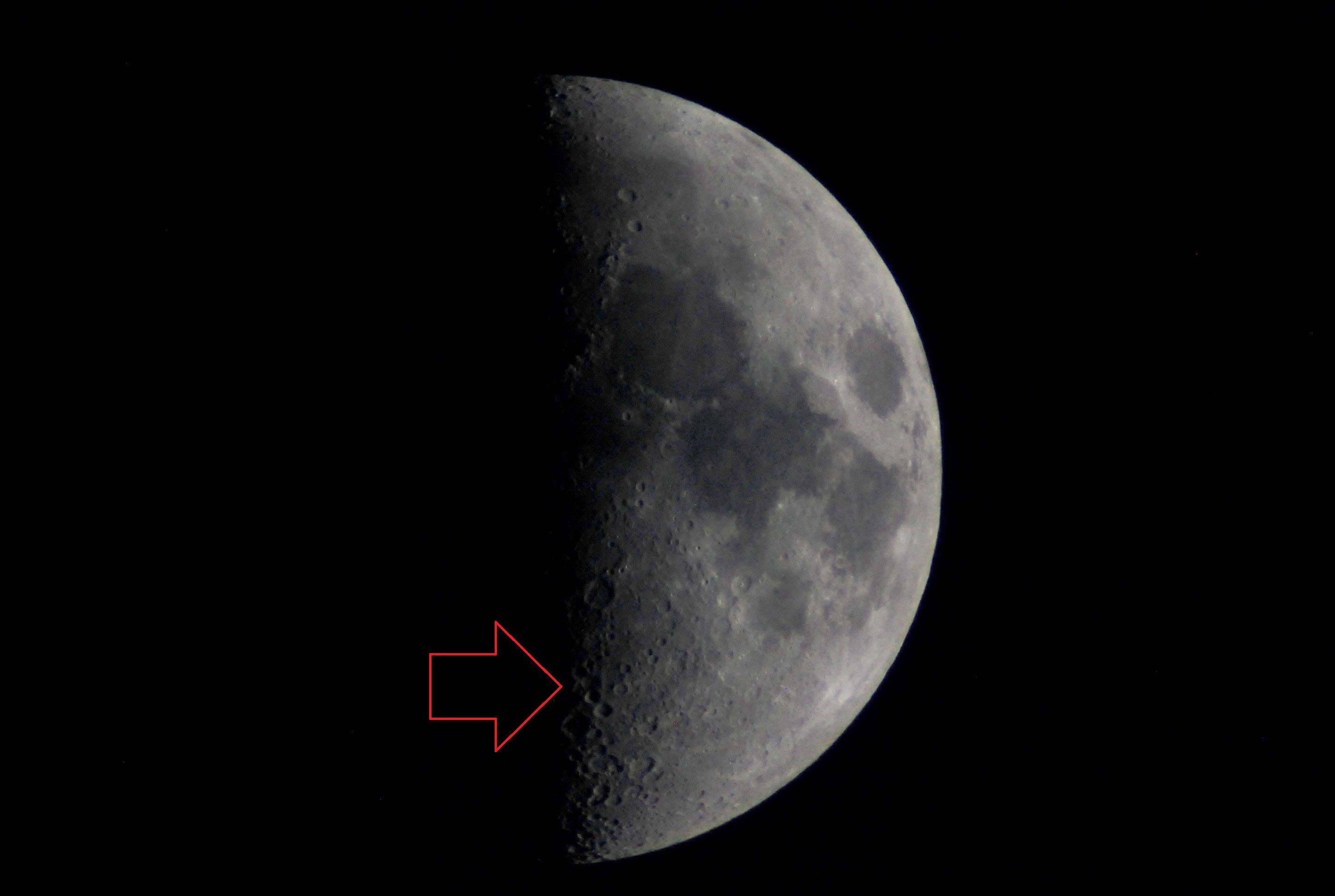
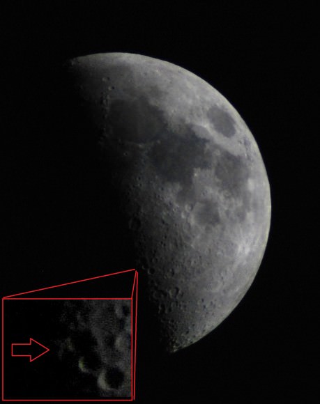
This week, we get a unique look at a feature embedded in the lunar highlands which demonstrates this fact. The Lunar X, also sometimes known as the Purbach cross or the Werner X reaches a decent apparition on March 19th at 11:40UT/7:40EDT favoring East Asia and Australia. This feature is actually the overlapping convergence of the rims of Blanchinus, La Caille and Purbach craters. The X-shaped feature reaches a favorable illumination about six hours before 1st Quarter phase and six hours after Last Quarter phase. It is pure magic watching the X catch the first rays of sunlight while the floor of the craters are still immersed in darkness. For about the span of an hour, the silver-white X will appear to float just beyond the lunar terminator.

Visibility of the Lunar X for the Remainder of 2013.

Lunation Date Time Phase Favors
1116 March 19th 11:40UT/7:40EDT Waxing East Asia/Australia
1116 April 3rd 3:20UT/23:20EDT* Waning Africa/Europe
1117 April 17th 23:47UT/19:47EDT Waxing Eastern North America
1117 May 2nd 16:19UT/12:19EDT Waning Central Pacific
1118 May 17th 10:51UT/6:51EDT Waxing East Asia/Australia
1118 June 1st 4:31UT/0:31EDT Waning Western Africa
1119 June 15th 21:21UT/17:21EDT Waxing South America
1119 June 30th 16:04UT/12:04EDT Waning Western Pacific
1120 July 15th 7:49UT/3:49EDT Waxing Australia
1120 July 30th 3:16UT/23:16EDT* Waning Africa/Western Europe
1121 August 13th 18:50UT/14:50EDT Waxing South Atlantic
1121 August 28th 14:27UT/10:27EDT Waning Central Pacific
1122 September 12th 9:50UT/5:50EDT Waxing East Asia/Australia
1122 September 27th 2:00UT/22:00EDT* Waning Middle East/East Africa
1123 October 11th 19:52UT/15:52EDT Waxing Atlantic Ocean
1123 October 26th 14:12UT/10:12EDT Waning Central Pacific
1124 November 10th 10:03UT/5:03EST Waxing East Asia/Australia
1124 November 25th 3:14UT/22:14EST* Waning Africa/Europe
1125 December 10th 00:57UT/19:57EST Waxing Western North America
1126 December 24th 17:07UT/12:07EST Waning Western Pacific
*Times marked in bold denote visibility in EDT/EST the evening prior.


Fun Factoid: All lunar apogees and perigees are not created equal either. The Moon also reaches another notable point tonight at 11:13PM EDT/ 3:13 UT as it arrives at its closest apogee (think “nearest far point”) in its elliptical orbit for 2013 at 404,261 kilometres distant. Lunar apogee varies from 404,000 to 406,700 kilometres, and the angular diameter of the Moon appears 29.3’ near apogee versus 34.1’ near perigee. The farthest and visually smallest Full Moon of 2013 occurs on December 17th.

The first sighting of the Lunar X feature remains a mystery, although modern descriptions of the curious feature date back to an observation made by Bill Busler in June 1974. As the Sun rises across the lunar highlands the feature loses contrast. By the time the Moon reaches Full, evidence of the Lunar X vanishes all together. With such a narrow window to catch the feature, many longitudes tend to miss out during successive lunations. Note that it is possible to catch the 1st and Last Quarter Moon in the daytime.

A 1st Quarter Moon with the Lunar X (inset). (Photo by Author).

Compounding the dilemma is the fact that the lighting angle for each lunation isn’t precisely the same. This is primarily because of two rocking motions of the Moon known as libration and nutation. Due to these effects, we actually see 59% of the lunar surface. We had to wait for the advent of the Space Age and the flight of the Soviet spacecraft Luna 3 in 1959 to pass the Moon and look back and image its far side for the first time.

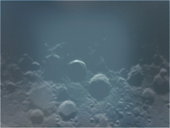
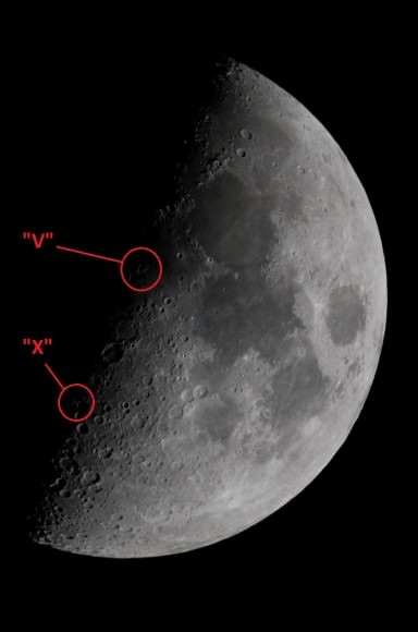
We actually managed to grab the Lunar X during a recent Virtual Star Party this past February. Note that another fine example of lunar pareidolia lies along the terminator roughly at the same time as the Lunar X approaches favorable illumination. The Lunar V sits near the center of the lunar disk near 1st and Last Quarter as well and is visible right around the same time. Formed by the confluence of two distinct ridges situated between the Mare Vaporum and Sinus Medii, it is possible to image both the Lunar X and the Lunar V simultaneously!

A simultaneous capture of the Lunar X & the Lunar V features. (Photo by Author).

This also brings up the interesting possibility of more “Lunar letters” awaiting discovery by keen-eyed amateur observers… could a visual “Lunar alphabet be constructed similar to the one built by Galaxy Zoo using galactic structures? Obviously, the Moon has no shortage of “O’s,” but perhaps “R” and “Q” would be a bit more problematic. Let us know what you see!

-Thanks to Ed Kotapish for providing us with the calculations for the visibility of the Lunar X for 2013.


A Weekend of Comet PANSTARRS: Spectacular Images and Videos

Comet PANSTARRS above a farm near Alto, Michigan. Credit: Kevin's Stuff on Flickr.

Comet C/2011 L4 (PanSTARRS) keeps getting easier to see, and over the weekend, we were inundated with images and videos from astrophotographers around the world. NASA says that solar heating from the comet’s close pass of the Sun last week has caused the comet to glow brighter than a first magnitude star. Bright twilight sharply reduces visibility, but it is still an easy target for binoculars and small telescopes 1 and 2 hours after sunset. And as of March 15th, people reported they can see the comet with the unaided eye.

See more images and videos below!

Timelapse of comet Panstarrs from Leiden Observatory from Fred Kamphues on Vimeo.

Photographer Fred Kamphues took this timelapse from the Leiden Observatory in The Netherlands, the oldest astronomical observatory in the world still active today. Kamphues notes that astronomer Jan Hendrik Oort of Leiden Observatory discovered the origin of comets in 1950. The observatory is used today by student astronomers to learn observing.

Comet C/2011 L4 (PANSTARRS) taken on March 16 from Mount Faito (Naples, Italy). Credit and copyright: Ernesto Guido & Antonio Catapano
Special filters and a negative image to try and 'tease out the structure of the tail,' says photographer David G. Strange.
Special filters and a negative image to try and ‘tease out the structure of the tail,’ says photographer David G. Strange.
Comet PANSTARRS over Tallinn, Estonia on March 16, 2013.  Credit and copyright: Karthikeyan VJ
Comet PANSTARRS over Tallinn, Estonia on March 16, 2013.
Credit and copyright: Karthikeyan VJ
Comet PANSTARRS over the San Gabriel mountains on 3/12/2013 above Pasadena,CA,  3-4 miles from Mt.Wilson. Shot with a with Canon 60D. Credit and copyright: Henry Levenson.
Comet PANSTARRS over the San Gabriel mountains on 3/12/2013 above Pasadena,CA, 3-4 miles from Mt.Wilson. Shot with a with Canon 60D. Credit and copyright: Henry Levenson.
Comet PANSTARRS, shot from near Keene, Ontario, Canada, on March 16, 2013, using a Canon 50D (modified) with Canon 200mm lens; 4 sec. exp.; f/4.5; 640 ISO. Credit and copyright: Rick Stankiewicz, Peterborough Astronomical Association (PAA)
[/caption

This video, above, from UT reader Brent (a.k.a. HelloBozos) in Florida shows this compilation of views of the Sun and the comet. “At 2:08 in the video, a bird flies in front of the camera,” Brent said via email, “This was all done off the side the road, on 3-16-13 8pm-8:30pm.”

[caption id="attachment_100801" align="aligncenter" width="580"]Comet PANSTARRS over Arizona on March 16, 2013. Credit and copyright: Chris Schur Comet PANSTARRS over Arizona on March 16, 2013. Credit and copyright: Chris Schur

This image is from Chris Schur in Arizona. He says, “Note the fan tail appearing! Also the tail is really starting to curve in the images. Very easy to see naked eye, and so was the yellow color in binoculars when it gets lower.”

Comet PANSTARRS on March 17, 2013. Credit and copyright: Andrei Juravle.
Comet PanSTARRS (C/2011 L4) taken near Koprivnica (Koprivni?ki Bregi), Croatia. Credit and copyright: Vedran Matica.

5 Mercury Secrets Revealed by MESSENGER

Artist's concept of MESSENGER in orbit around Mercury. Courtesy of NASA

After two years of doing the loop-the-loop around Mercury, MESSENGER has unveiled a bunch of surprises from Mercury — the closest planet to the Sun.

The spacecraft launched in 2004 and made three flybys of the planet before settling into orbit two years ago today. Incredibly, MESSENGER is only the second NASA probe to visit Mercury; the first one, Mariner 10, only flew by a few times in the 1970s. It was an incredible feat for the time, but we didn’t even have a complete map of Mercury before MESSENGER arrived at the planet.

So, what have scientists found in MESSENGER’s two years in orbit? Tales of sulfur, organic materials and iron, it turns out.

Mercury’s south pole has a weak spot

Magnetic field lines differ at Mercury's north and south poles As a result of the north-south asymmetry in Mercury's internal magnetic field, the geometry of magnetic field lines is different in Mercury's north and south polar regions. Credit: NASA/Johns Hopkins University Applied Physics Laboratory/Carnegie Institution of Washington
Magnetic field lines differ at Mercury’s north and south poles As a result of the north-south asymmetry in Mercury’s internal magnetic field, the geometry of magnetic field lines is different in Mercury’s north and south polar regions. Credit: NASA/Johns Hopkins University Applied Physics Laboratory/Carnegie Institution of Washington

The magnetic field lines converge differently at the north and south poles of Mercury. What does this mean? There’s a larger “hole” at the south pole for charged particles to do their thing to the surface of Mercury. At the time this information was released, NASA said it’s possible that space weathering or erosion would be different at the north and south poles because of this. Charged particles on the surface would also add to Mercury’s wispy atmosphere.

How the atmosphere changes according to distance from the sun

Comparison of neutral sodium observed during MESSENGER’s second and third Mercury flybys
Comparison of neutral sodium observed during MESSENGER’s second and third Mercury flybys. Credit: NASA

Wondering about the atmosphere on Mercury? It depends on the season, and also the element. The scientists found striking changes in calcium, magnesium and sodium when the planet was closer to and further from the sun.

“A striking illustration of what we call ‘seasonal’ effects in Mercury’s exosphere is that the neutral sodium tail, so prominent in the first two flybys, is 10 to 20 times less intense in emission and significantly reduced in extent,” said participating scientist Ron Vervack, of the Johns Hopkins University Applied Physics Laboratory in 2009. “This difference is related to expected variations in solar radiation pressure as Mercury moves in its orbit and demonstrates why Mercury’s exosphere is one of the most dynamic in the solar system.”

Discovery of water ice and organics

A radar image of Mercury’s north polar region is shown superposed on a mosaic of MESSENGER images of the same area. All of the larger polar deposits are located on the floors or walls of impact craters. Deposits farther from the pole are seen to be concentrated on the north-facing sides of craters. Credit: NASA/Johns Hopkins University Applied Physics Laboratory/Carnegie Institution of Washington/National Astronomy and Ionosphere Center, Arecibo Observatory

Late in 2012, NASA finally was able to corroborate some science results from about 20 years ago. Scientists on Earth saw “radar bright” images from Mercury in the 1990s, implying that there was ice and organic materials at the poles. MESSENGER finally confirmed that through three separate lines of investigation that were published in Science in 2012. Scientists estimated the planet holds between 100 billion and 1 trillion tons of water ice, perhaps as deep as 20 meters in some places. “Water ice passed three challenging tests and we know of no other compound that matches the characteristics we have measured with the MESSENGER spacecraft,” said MESSENGER principal investigator Sean Solomon in a NASA briefing.

Mercury has a big iron core

The internal structure of Mercury is very different from that of the Earth. The core is a much larger part of the whole planet in Mercury and it also has a solid iron-sulfur cover. As a result, the mantle and crust on Mercury are much thinner than on the Earth.  Credit: Case Western Reserve University
The internal structure of Mercury is very different from that of the Earth. The core is a much larger part of the whole planet in Mercury and it also has a solid iron-sulfur cover. As a result, the mantle and crust on Mercury are much thinner than on the Earth.
Credit: Case Western Reserve University

While scientists knew before that Mercury has an iron core, the sheer size of it surprised scientists. At 85%, the proportion of the core to the rest of the planet dwarfs its rocky solar system companions. Further, scientists measured Mercury’s gravity. From that, they were surprised to see that the planet had a partially liquid core. “The planet is sufficiently small that at one time many scientists thought the interior should have cooled to the point that the core would be solid,” stated Case Western Reserve University’s Steven A. Hauck II, a co-author of a paper on the topic that appeared in Science Express.

The surface is sulfur-rich

A global view of Mercury, as seen by MESSENGER. Credit: NASA

At some point in Mercury’s history, it’s possible that it could have had lavas erupt and sprinkle the surface with sulfur, magnesium and similar materials. At any rate, what is known for sure is there is quite a bit of sulfur on Mercury’s surface. “None of the other terrestrial planets have such high levels of sulfur. We are seeing about ten times the amount of sulfur than on Earth and Mars,” said paper author Shoshana Weider of the Carnegie Institution of Washington.

What Glows Green In Space?

The Wreath Nebula (Barnard 3) glows green in space in this Wide-field Infrared Survey Explorer (WISE) image. Credit: NASA/JPL-Caltech/UCLA

While a quest for green beer in space would be difficult, we’re happy to report there are other ways you can celebrate Saint Patrick’s Day while looking at the night sky. Just check out the nebulae and aurorae in these pictures!

A word of caution, these pictures are taken by cameras that expose light for a very long time, sometimes using different filters, to bring out the colors. A nebula, for example, seen with our own eyes does not look quite as stunning.

The picture above shows the Wreath Nebula, which apparently is filled with warm dust bits that are about the same composition as smog.

RCW 120. Credit: NASA/JPL-Caltech

Here’s a picture of a “Green Ring” Nebula; the NASA press release is worth a read for the hilarious Green Lantern references. But besides the science fiction, there is some neat science in action here: “The green color represents infrared light coming from tiny dust grains called polycyclic aromatic hydrocarbons,” NASA writes. “These small grains have been destroyed inside the bubble. The red color inside the ring shows slightly larger, hotter dust grains, heated by the massive stars.”

A portion of the Lagoon nebula imaged by the Gemini South telescope with the Gemini Multi-Object Spectrograph. Credit: Julia I. Arias and Rodolfo H. Barbá Departamento de Física, Universidad de La Serena (Chile), and ICATE-CONICET (Argentina).

You can even see hints of green in the Lagoon Nebula picture above. Using a filter that picks up green (sulfur) emission, the astronomers ferreted out a bit of emerald.

An October 2012 picture from Jason Arhns in Alaska, which he calls a “ghost flame.” Credit: Jason Arhns

If you live far enough north or south, you occasionally get to see aurorae dancing across the sky. These events, sometimes known as the Northern Lights or Southern Lights, occur due to interactions between the sun’s particles and the Earth’s upper atmosphere. We had some green stunners in October 2012 after a solar flare pushed a bunch of these particles in Earth’s direction. Most of the light you see in auroras comes from oxygen atoms being “excited” from the interaction with the sun’s particles; green occurs at higher altitudes, and red at lower ones.

Light curve of different stars.

One object that can’t glow green in space, however, is a star. Stellar colors depend on the surface of the star. Blue stars, the hottest ones, are at about 12,000 Kelvin and red stars, the coolest ones, are less than 3,500 Kelvin. (The sun is about in the middle, at 6,800 Kelvin, as it emits white light.)

As Universe Today publisher Fraser Cain pointed out in a past post, the only way a green star could be possible is if the light curve peaks at green. That doesn’t work, however: “If you make the star hotter, it just gets bluer,” he wrote. “And if you make a star cooler, it just becomes orange and then redder. There’s no way to have a light curve that makes a star look green.” Check out more details here.

Comet Pan-STARRS Wows Over Holland

Comet Pan-STARRS thrills Dutch observers of the Night Sky on March 15, 2013 shortly after sunset. Shot with a Canon 60D camera and Canon 100/400 mm lens, exposure time 15 seconds, ISO 300 Credit: Rob van Mackelenbergh

Comet Pan-STARRS thrills Dutch observers of the Night Sky on March 14, 2013 shortly after sunset- note the rich hues. Shot with a Canon 60D camera and Canon 100/400 mm lens, exposure time 2 seconds, ISO 800. Credit: Rob van Mackelenbergh
See viewing guide and sky maps below
Update – see readers photo below[/caption]

Comet Pan-STARRS (C/2011 L4) is exciting amateur astronomers observing the night sky worldwide as it becomes visible in the northern latitudes after sunset. And now it’s wowing crowds in Europe and all over Holland – north to south.

Check out the beautiful, richly hued new photos of Comet Pan-STARRS captured on March 14, 2013 by Dutch astrophotographer Rob van Mackelenbergh.

“I took these photos in the southern part of the Netherlands on Thursday evening, March 14, at around 7:45 pm Dutch time with my Canon 60 D camera.”

“I was observing from the grounds of our astronomy club – “Sterrenwacht Halley” – named in honor of Halley’s Comet.”

Comet Pan-STARRS is a non-periodic comet from the Oort Cloud that was discovered in June 2011 by the Pan-STARRS telescope located near the summit of the Hawaiian Island of Maui.

The comet just reached perihelion – closest approach to the Sun – on March 10, 2013. It passed closest to Earth on March 5 and has an orbital period of 106,000 years.

Comet Pan-STARRS from Holland on March 15, 2013 at about 7:45 PM, shortly after sunset - Canon 60D camera, Canon 100/400 mm lens, exposure time 15 seconds, ISO 300.   Credit: Rob van Mackelenbergh
Comet Pan-STARRS from Holland on March 14, 2013 at about 7:45 PM, shortly after sunset – Canon 60D camera, Canon 100/400 mm lens, exposure time 2 seconds, ISO 800. Credit: Rob van Mackelenbergh

“Over 30 people were watching with me and they were all very excited, looking with binoculars and cameras. People were cheering. They were so excited to see the comet. But it was very cold, about minus 2 C,” said Mackelenbergh.

The “Sterrenwacht Halley” Observatory was built in 1987 and houses a Planetarium and a Celestron C14 Schmidt-Cassegrain telescope. It’s located about 50 km from the border with Belgium, near Den Bosch – the capitol city of southern Holland.

Comet Pan-STARRS was photographed from Sterrenwacht Halley - or 'Halley Observatory' in Holland.  Credit: Rob van Mackelenbergh
Comet Pan-STARRS was photographed from Sterrenwacht Halley – or ‘Halley Observatory” in Holland. Credit: Rob van Mackelenbergh

“It was hard to see the comet with the naked eye. But we were able to watch it for about 45 minutes altogether in the west, after the sun set.”

“The sky was completely clear except for a few scattered clouds near the horizon. After the comet set, we went inside the observatory for a general lecture about Comets and especially Comets Pan-STARRS and ISON because most of the people were not aware about this year’s pair of bright comets.”

“So everyone was lucky to see Comet Pan-STARRS because suddenly the sky cleared of thick clouds!”

Comet Pan-STARRS from Holland on March 15, 2013 at about 7:45 PM, shortly after sunset - Canon 60D camera, Canon 100/400 mm lens, exposure time 15 seconds, ISO 300.   Credit: Rob van Mackelenbergh
Comet Pan-STARRS from Holland on March 14, 2013 at about 7:45 PM, shortly after sunset – Canon 60D camera, Canon 100/400 mm lens, exposure time 2 seconds, ISO 800. Credit: Rob van Mackelenbergh

“In the past I also saw Comet Halley and Comet Hale-Bopp, but these are my first ever comet photos and I’m really excited !”

“I hope to see Comet Pan-STARRS again in the coming days when the sky is clear,” Mackelenbergh told me.

Over the next 2 weeks or so the sunset comet may grow in brightness even as it recedes from Earth into darker skies. Right now it’s about magnitude 0.2.

So keep looking with your binoculars; look west for up to 1 to 2 hours after sunset – and keep your eyes peeled.

And report back here !

Ken Kremer


See a readers photo of sunset Comet Pan-STARRS below

Comet Pan-STARRS viewing graphic from NASA
Comet Pan-Starrs Sky Map. Viewing guide to find the comet low in the horizon after sunset.Credit: Space Weather.com
Comet Pan-Starrs Sky Map. Viewing guide to find the comet low in the horizon after sunset.Credit: Spaceweather.com

Phases of the Moon App Giveaway for iOS

Phases of the Moon

Enter to win a free copy of the Phases of the Moon App brought to you by Universe Today.

We’re giving away 10 copies of Phases of the Moon for iPhone/iPad.

Want to know the current phase of the Moon at all times? Perhaps you need to do some stargazing or astrophotography, or you really need to debunk some nonsense theories about full Moon madness… then check out our handy mobile app – available on iPhone or Android.

Here are the features:

  • Beautiful images of the Moon were made by NASA from data collected by the Lunar Reconnaissance Orbiter.
  • Full internal simulation of the Moon’s position and phase. See the current date, phase name, distance and illumination percentage.
  • Swipe left and right to move forward or backwards in time to see what the Moon will look like in the future or past.
  • Click a button to take you to the next full Moon.
  • You can also access a calendar that shows you the phase of the Moon for any date in the future.
  •  New 2013 features include total lunar eclipses, live Wallpaper and Widgets (for Android), and social sharing

The latest version of the app is running a full model of the Moon’s orbit and phases, displaying a scientifically accurate simulation of the Moon’s exact phase, size, distance and amount of illumination.

interfaceWe’ve just done a major update to the app, extending the support to iPhone, and completely rebuilding the Android edition to be smoother and more stable on the wide range of devices.

You can swipe the Moon back and forth to see how the Moon’s distance and illumination change over time, or jump to the next full Moon, or see the Moon’s phase at any point in the future. The Android version is especially smooth, and kind of hypnotic as you change the phase.

In order to be entered into the giveaway drawing, just put your email address into the box at the bottom of this post (where it says “Enter the Giveaway”) before Saturday, March 23, 2013. We’ll send you a confirmation email, so you’ll need to click that to be entered into the drawing.

Thank you for your interest. This giveaway is now closed.

If you are not lucky enough to win a promo code, you can purchase a copy for $.99 on either Google Play or the iTunes Store, and help support Universe Today.

Kepler Team Identifies Planet Impostors that are Binary Stars in Disguise

A new study describes how the Kepler team aims to remove pseudo-planets from its database. A pseudo-planet can be caused by the superposition of a foreground bright constant target star, and background fainter multiple star systems as shown in the above artist sketch (image credit: regulus36/devianart).

Observations by the Kepler satellite have advanced our knowledge of stars and their orbiting planets, yielding more than 100 confirmed planets and about 3,000 candidates.  However, orbiting planets may not be the source for a fraction of those detections.

“There are many things in the sky that can produce transit-like signals that are not planets, and thus we must be sure to identify what really is a planet detected by Kepler,” Stephen Bryson told Universe Today.  NASA Ames Research Center scientists Bryson and Jon Jenkins (also at the SETI Institute) are the lead authors on a new paper that aims to identify pseudo-planets detected by Kepler.

Small eclipses present in Kepler brightness measurements for a star (a lightcurve) may be indicative of an orbiting planet blocking light from its host star (see image below).  However, under certain circumstances binary stars can mimic that signature.

Consider a Kepler target that is actually a chance superposition of a bright star and a fainter eclipsing binary system, whereby the objects lie at different distances along the sight-line.  The figure below illustrates that their combined light can produce a lightcurve that is similar to a transiting planet.  The bright foreground star dilutes the typically large eclipses produced by the binary system.

Left, the lightcurve for a star featuring a transiting planet, whereby the planet blocks a minute fraction of the host star’s light (image credit: Institute for Astronomy, University of Hawaii at Manoa).  Right, the combined light from a foreground bright star and a fainter eclipsing binary system can mimic a transiting planet (image credit: chart and assembly, D. Majaess – cropped stellar graphics from Collier Cameron 2012, Nature).

“Most of the time these eclipsing binaries are not exactly aligned with our target star,” Bryson added, “and we can carefully examine the pixels to discover that the location of the transit signal is not the target star.”  The team developed algorithms to identify pseudo-planets when the stars are individually resolved.  Tagging spurious planet detections is important since there are numerous candidates, and yet limited observing time for follow-up efforts.

The team has been refining those algorithms as knowledge of the satellite’s in situ behavior increases.  “These algorithms have been developed and used over the last four years.  Some details of the techniques in the paper are new and will appear in future versions of the Kepler [software processing] pipeline,” said Bryson.

However, if multiple stars fall within the same pixel they are not individually resolved by Kepler, and a separate approach is required to infer their presence.  Consider the example highlighted in the image below, where several stars were unresolved by Kepler yet appear in higher resolution images.  The matter is exacerbated in part because Kepler’s spatial resolution is not optimal, and thus multiple stars may be confused as a single object.  By contrast, certain ground-based telescopes can achieve ~20 times Kepler’s spatial resolution when adaptive optics are implemented.

High-resolution images (right panel) can reveal stars that were unresolved in lower-resolution images (left panel, e.g., Kepler).   Unresolved stars dilute eclipses caused by transiting planets, and in certain cases can strongly bias the derived parameters (image credit: right panel from Adams et al. 2012, arXiv/AJ – left panel, image blurred to provide a lower-resolution glimpse of the target, assembly by D. Majaess).

Adams et al. 2012 obtained high-resolution images of 90 Kepler targets, one of which is highlighted above.  That team noted that, “Close companions … are of particular concern … Of the [90 Kepler targets surveyed] 20% have at least one companion within [half a Kepler pixel].”  The high-resolution images were acquired via the MMT observatory (shown below) and the Palomar Hale-200-inch telescope.

Obviously, the resolution problem becomes more acute when observing rich stellar fields (high densities), such as near the plane of our Galaxy.   

“Background eclipsing binaries account for as many as 35% of all planet-like transit signals when we are looking near the Milky Way, because there are many stars in the background,” Bryson told Universe Today. “When we look away from the Milky Way the fraction of background eclipsing binaries falls to about 10% of all planet-like transit signals because there are far fewer background stars of all types.”

However, regarding Kepler’s coarser resolution Bryson underscored that, “[it is] expected with such a large field telescope.” Kepler’s large field is certainly advantageous, as it permits the satellite to monitor 100,000+ stars over more than 100 square degrees of field.

The adaptive optics (AO) system at the MMT observatory provides astronomers with high-resolution images to search the vicinity of Kepler planet candidates for contaminating stars (image credit: Thomas Stalcup, SPIE).

Radial velocity measurements are an ideal means for evaluating planet candidates (and to help yield the mass).  The data are pertinent since velocity shifts occur in the spectrum of the host star owing to the planet’s gravity.  However, Adams et al. 2012 note that “Many of these objects do not have … radial velocity measurements because of the amount of observing time required, particularly for small planets around relatively faint stars. Another method is needed to confirm these types of planets … High-resolution images are thus a crucial component of any transit follow-up program.”

Identifying unresolved stars is crucial for yet another reason.  Note that the fundamental parameters determined for a transiting planet depend in part on the fraction of the host star’s light that is obscured (the eclipse depth).  However, if multiple unresolved stars exist they will contribute to the overall brightness, and hence the observed planet eclipse will be diluted and underestimated (see figure 2, above).  Indeed, Adams et al. 2012 note that, “Corrections to the planetary parameters based on nearby [contaminating] stars can range from a few to tens of percents, making high resolution images an important tool to understanding the true sizes of other discovered worlds.”

The case of K00098 is a prime example underscoring the importance of identifying unresolved contaminating stars.   K00098 features two rather bright stars that were unresolved and unknown prior to the acquisition of high-resolution images. Consequently, previously determined parameters for that star’s transiting planet were incorrect. Concerning K00098, Adams et al. 2012 remarked that, “for K00098, the dilution [of the eclipse depth] … were substantial: the [planet’s] radius increased by 10%, the mass by 60% … and the density changed by 25% [from that published]. Without high resolution images, we would have had a very inaccurate picture of this planet.”

Low and high-resolution images of stars in the galaxy M33. The bright object detected in the low-resolution image is actually several stars, as indicated by the higher-resolution image. A similar effect occurs when comparing Kepler (lower-resolution) and AO images (higher-resolution). A single Kepler target can actually constitute multiple stars seen along the sight-line (image credit: Mochejska et al. 2001, arXiv).
Low and high-resolution images of stars in the galaxy M33. The bright object detected in the low-resolution image is actually several stars, as indicated by the higher-resolution image (right). A similar effect occurs when comparing Kepler (lower-resolution) and AO images (higher-resolution). A single Kepler target can actually constitute multiple stars seen along the sight-line (image credit: Mochejska et al. 2001, arXiv).

Incidentally, unaccounted for light from unresolved stars isn’t merely a problem for exoplanet studies.  The issue is rather pertinent when researching the cosmic distance scale and the Hubble constant (expansion rate of the Universe).  Consider the images above which feature the same field in M33.  The image exhibited on the left is from a ground-based facility, whereas the higher-resolution image displayed on the right is from the Hubble Space Telescope (HST).  The brightest star at the center of the image is a Cepheid variable star, which is a pulsating star that is used to establish distances to galaxies.  In turn those distances are subsequently employed to determine the Hubble constant.  The HST image reveals stars that are unresolved in the ground-based image, and thus the distance inferred from that observation is compromised since the Cepheid appears (spuriously) brighter than it should be.

“Blending [e.g., added light caused by unresolved stars] leads to systematically low distances to galaxies observed with the HST, and therefore to systematically high estimates of the Hubble constant,” remarked Mochejska et al. 2004.  However, there is an ongoing debate concerning the importance of such an effect (Ferrarese et al. 2000, Mochejska et al. 2001).

In sum, numerous groups are developing methods to identify pseudo-planets in the Kepler database.  Given the large sample and sizable investment of time required to confirm a planet candidate: such efforts are important (e.g., Bryson et al. 2013).  Data from the Kepler mission have helped advance our understanding of stars and their orbiting planets, and more is yet to come.  If you’d like to help the Kepler team identify planets around other stars: join the Planet Hunters citizen science project.

The Bryson et al. 2013 findings have been submitted to PASP for peer review, and a preprint is available on arXiv.  The coauthors on the study are J. Jenkins, R. Gilliland, J. Twicken, B. Clarke, J. Rowe, D. Caldwell, N. Batalha, F. Mullally, M. Haas, and P. Tenenbaum.  The interested reader desiring additional information will find the following pertinent:  Adams et al. 2012Collier Cameron 2012 (e.g., for other scenarios that can mimic the lightcurve of a transiting-planet), “Strange New Worlds: The Search for Alien Planets and Life beyond Our Solar System” by Ray Jayawardhana, “Distant Wanderers: The Search for Planets Beyond the Solar System” by Bruce Dorminey.  For discussion on how light from unresolved sources affects the cosmic distance scale see Mochejska et al. 2004 (and for the opposite point of view, and subsequent rebuttal: Ferrarese et al. 2000Mochejska et al. 2001).

Survival: Terrifying Moments in Space Flight

Apollo 13's dangerous explosion in 1970 inspired a movie, released in 1995, that starred (left to right) Bill Paxton, Kevin Bacon and Tom Hanks. Credit: Universal Pictures

Space is a dangerous and sometimes fatal business, but happily there were moments where a situation happened and the astronauts were able to recover.

An example: today (March 16) in 1966, Neil Armstrong and Dave Scott were just starting the Gemini 8 mission. They latched on to an Agena target in the hopes of doing some docking maneuvers. Then the spacecraft started spinning inexplicably.


They undocked and found themselves tumbling once per second while still out of reach of ground stations. A thruster was stuck open. Quick-thinking Armstrong engaged the landing system and stabilized the spacecraft. This cut the mission short, but saved the astronauts’ lives.

Gemini 8's Agena target before a stuck thruster on the spacecraft put the astronauts in a terrifying tumble. Credit: NASA
Gemini 8’s Agena target before a stuck thruster on the spacecraft put the astronauts in a terrifying tumble. Credit: NASA

Here are some other scary moments that astronauts in space faced, and survived:

Friendship 7: False landing bag indicator (1962)

Astronaut John Glenn views stencilling used as a model to paint the words "Friendship 7" on his spacecraft. Credit: NASA
Astronaut John Glenn views stencilling used as a model to paint the words “Friendship 7” on his spacecraft. Credit: NASA

John Glenn was only the third American in space, so you can imagine the amount of media attention he received during his three-orbit flight. NASA received an indication that his landing bag had deployed while he was still in space. Friendship 7’s Mercury spacecraft had its landing cushion underneath the heat shield, so NASA feared it had ripped away. Officials eventually informed Glenn to keep his retrorocket package strapped to the spacecraft during re-entry, rather than jettisoning it, in the hopes the package would keep the heat shield on. Glenn arrived home safely. It turned out to be a false indicator.

Apollo 11: Empty fuel tank (1969)

Apollo 11's Eagle spacecraft, as seen from fellow spaceship Columbia. Credit: NASA
Apollo 11’s Eagle spacecraft, as seen from fellow spaceship Columbia. Credit: NASA

Shortly after Neil Armstrong announced “Houston, Tranquility Base, here, the Eagle has landed” during Apollo 11, capsule communicator Charlie Duke answered, “Roger, Tranquility. We copy you on the ground. You got a bunch of guys about to turn blue. We’re breathing again. Thanks a lot.” They weren’t holding their breath just because it was the first landing on the moon; Armstrong was navigating a spacecraft that was almost out of fuel. The spacecraft Eagle overshot its landing and Armstrong did a series of maneuvers to put it on relatively flat ground. Accounts say he had less than 30 seconds of fuel when he landed on July 20, 1969.

Apollo 12: Lightning strike (1969)

Apollo 12's launch in 1969, moments before the rocket was struck by lightning. Credit: NASA
Apollo 12’s launch in 1969, moments before the rocket was struck by lightning. Credit: NASA

Moments after Apollo 12 headed from ground towards orbit, a lightning bolt hit the rocket and caused the spacecraft to go into what appeared to be a sort of zombie mode. The rocket was still flying, but the astronauts (and people on the ground) were unsure what to do. Scrambling, one controller suggested a command that essentially reset the spacecraft, and Apollo 12 was on its way. NASA did take some time to do some double-checking in orbit, to be sure, before carrying on with the rest of the mission. The agency also changed procedures about launching in stormy weather.

Apollo 13: Oxygen tank explosion (1970)

Evidence of the Apollo 13 explosion on the spacecraft Odyssey. Credit: NASA
Evidence of the Apollo 13 explosion on the service module. Credit: NASA

The astronauts of Apollo 13 performed a routine stir of the oxygen tanks on April 13, 1970. That’s when they felt the spacecraft shudder around them, and warning lights lit up. It turned out that an oxygen tank, damaged through a series of ground errors, had exploded in the service module that fed the spacecraft Odyssey, damaging some of its systems. The astronauts survived for days on minimal power in Aquarius, the healthy lunar module that was originally supposed to land on the moon. They arrived home exhausted and cold, but very much alive.

Apollo-Soyuz Test Project: Toxic vapours during landing (1975)

The Apollo command module used in the Apollo-Soyuz Test Project, during recovery. Credit: NASA

The Apollo-Soyuz Test Project was supposed to test out how well American and Russian systems (and people) would work together in space. Using an Apollo command module and a Russian Soyuz, astronauts and cosmonauts met in orbit and marked the first mission between the two nations. That almost ended in tragedy when the Americans returned to Earth and their spacecraft was inadvertently flooded with vapours from the thruster fuel. “I started to grunt-breathe to make sure I got pressure in my lungs to keep my head clear. I looked over at Vance [Brand] and he was just hanging in his straps. He was unconscious,” recalled commander Deke Slayton, in a NASA history book about the event. Slayton ensured the entire crew had oxygen masks, Brand revived quickly, and the mission ended shortly afterwards.

Mir: The fire (1997)

Jerry Linenger dons a mask during his mission on Mir in 1997. Credit: NASA

The crew on Mir was igniting a perchlorate canister for supplemental oxygen when it unexpectedly ignited. As they scrambled to put out the fire, NASA astronaut Jerry Linenger discovered at least one oxygen mask on board were malfunctioning as well. The crew managed to contain the fire quickly. Even though it affected life aboard the station for a while afterwards, the crew survived, did not need to evacuate, and helped NASA learn lessons that they still use aboard the International Space Station today.

STS-51F: Abort to orbit (1985)

STS-51F aborted to orbit during its launch. Credit: NASA

The crew of space shuttle Challenger endured two aborts on this mission. The first one took place at T-3 seconds on July 12, when a coolant valve in one of the shuttle’s engines malfunctioned. NASA fixed the problem, only to face another abort situation shortly after liftoff on July 29. One of the engines shut down too early, forcing the crew to abort to orbit. The crew was able to carry on its mission, however, including many science experiments aboard Spacelab.

STS-114: Foam hitting Discovery (2005)

Discovery during STS-114, as seen from the International Space Station. CREDIT: NASA

When Discovery lifted off in 2005, the fate of the entire shuttle program was resting upon its shoulders. NASA had implemented a series of fixes after the Columbia disaster of 2003, including redesigning the process that led to foam shedding off Columbia’s external tank and breaching the shuttle wing. Wayne Hale, a senior official in the shuttle program, later recalled his terror when he heard of more foam loss on Discovery: “I think that must have been the worst call of my life. Once earlier I had gotten a call that my child had been in an auto accident and was being taken to the hospital in an ambulance. That was a bad call. This was worse.” The foam, thankfully, struck nothing crucial and the crew survived. NASA later discovered the cracks in the foam are linked to changes in temperature the tank undergoes, and made more changes in time for a much more successful mission in 2006.

We’ve probably missed some scary moments in space, so which ones do you recall?

Expedition 34 Crew Gets a Foggy Welcome Home

Three members of the Expedition 34 crew undocked from the International Space Station a day later than originally planned on Friday due to bad weather in the landing area in Kazakhstan, but returned safely to Earth, despite continuing cold, foggy weather. The deteriorating weather conditions allowed only two of 12 search and rescue helicopters to land at the touchdown site because of heavy clouds and fog. NASA TV was unable to show the actual landing after the Soyuz capsule descended into the dense fog.
Continue reading “Expedition 34 Crew Gets a Foggy Welcome Home”

What Mount Sharp Would Look Like on Earth

Gale crater's central peak as it might look under Earthly lighting (NASA/JPL-Caltech/MSSS)

Ahh — there’s nothing like a beautiful sunny day in Gale crater! The rusty sand crunching beneath your wheels, a gentle breeze blowing at a balmy 6º C (43º F), Mount Sharp rising in the distance into a clear blue sky… wait, did I just say blue sky?

I sure did. But no worries — Mars hasn’t sprouted a nitrogen-and-oxygen atmosphere overnight. The image above is a crop from a panoramic mosaic made of images from NASA’s Curiosity rover, showing Gale crater’s central peak Mount Sharp (or Aeolis Mons, if you prefer the official moniker.) Don’t let the blue sky fool you though — the lighting has been adjusted to look like a sunlit scene on Earth, if only to let geologists more easily refer to their own experience when studying the Martian landscape.

Click the image to see the full panorama, and a view of the same scene under more “natural” Martian lighting can be found below:

Aeolis Mons panorama seen in natural lighting (NASA/JPL-Caltech/MSSS)

According to JPL, in both versions the sky has been filled out by extrapolating color and brightness information from the portions of the sky that were captured in images of the terrain.

The elevation of Mt. Sharp compared to three mountains on Earth (NASA/JPL-Caltech/MSSS)

The component images were taken by the 100-millimeter-focal-length telephoto lens camera mounted on the right side of Curiosity’s remote sensing mast, during the 45th Martian day of the rover’s mission on Mars (Sept. 20, 2012).

Informally named after planetary scientist Robert Sharp by the MSL science team, the peak rises rises more than 3 miles (5 kilometers) above the floor of Gale crater.

See more news and images from the Curiosity rover here (and to find out what the latest weather conditions in Gale crater are visit MarsWeather.com here.)