Universe Today

March 16, 2013December 23, 2015 by Dan Majaess

Kepler Team Identifies Planet Impostors that are Binary Stars in Disguise

A new study describes how the Kepler team aims to remove pseudo-planets from its database. A pseudo-planet can be caused by the superposition of a foreground bright constant target star, and background fainter multiple star systems as shown in the above artist sketch (image credit: regulus36/devianart).

Observations by the Kepler satellite have advanced our knowledge of stars and their orbiting planets, yielding more than 100 confirmed planets and about 3,000 candidates. However, orbiting planets may not be the source for a fraction of those detections.

“There are many things in the sky that can produce transit-like signals that are not planets, and thus we must be sure to identify what really is a planet detected by Kepler,” Stephen Bryson told Universe Today. NASA Ames Research Center scientists Bryson and Jon Jenkins (also at the SETI Institute) are the lead authors on a new paper that aims to identify pseudo-planets detected by Kepler.

Small eclipses present in Kepler brightness measurements for a star (a lightcurve) may be indicative of an orbiting planet blocking light from its host star (see image below). However, under certain circumstances binary stars can mimic that signature.

Consider a Kepler target that is actually a chance superposition of a bright star and a fainter eclipsing binary system, whereby the objects lie at different distances along the sight-line. The figure below illustrates that their combined light can produce a lightcurve that is similar to a transiting planet. The bright foreground star dilutes the typically large eclipses produced by the binary system.

Left, the lightcurve for a star featuring a transiting planet, whereby the planet blocks a minute fraction of the host star’s light (image credit: Institute for Astronomy, University of Hawaii at Manoa). Right, the combined light from a foreground bright star and a fainter eclipsing binary system can mimic a transiting planet (image credit: chart and assembly, D. Majaess – cropped stellar graphics from Collier Cameron 2012, Nature).

“Most of the time these eclipsing binaries are not exactly aligned with our target star,” Bryson added, “and we can carefully examine the pixels to discover that the location of the transit signal is not the target star.” The team developed algorithms to identify pseudo-planets when the stars are individually resolved. Tagging spurious planet detections is important since there are numerous candidates, and yet limited observing time for follow-up efforts.

The team has been refining those algorithms as knowledge of the satellite’s in situ behavior increases. “These algorithms have been developed and used over the last four years. Some details of the techniques in the paper are new and will appear in future versions of the Kepler [software processing] pipeline,” said Bryson.

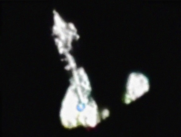
However, if multiple stars fall within the same pixel they are not individually resolved by Kepler, and a separate approach is required to infer their presence. Consider the example highlighted in the image below, where several stars were unresolved by Kepler yet appear in higher resolution images. The matter is exacerbated in part because Kepler’s spatial resolution is not optimal, and thus multiple stars may be confused as a single object. By contrast, certain ground-based telescopes can achieve ~20 times Kepler’s spatial resolution when adaptive optics are implemented.

High-resolution images (right panel) can reveal stars that were unresolved in lower-resolution images (left panel, e.g., Kepler). Unresolved stars dilute eclipses caused by transiting planets, and in certain cases can strongly bias the derived parameters (image credit: right panel from Adams et al. 2012, arXiv/AJ – left panel, image blurred to provide a lower-resolution glimpse of the target, assembly by D. Majaess).

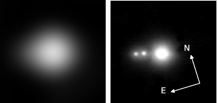
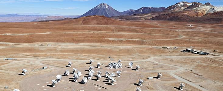
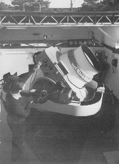
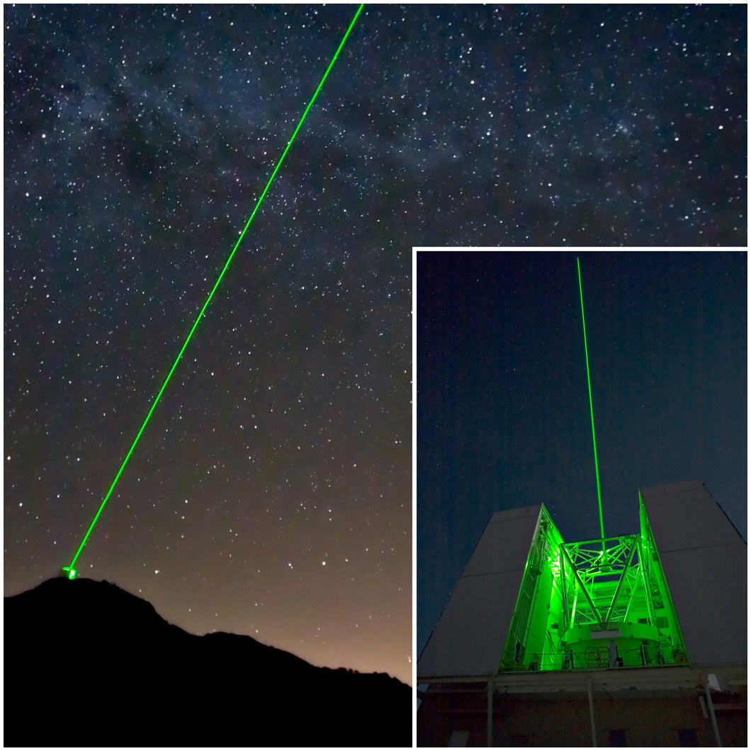
Adams et al. 2012 obtained high-resolution images of 90 Kepler targets, one of which is highlighted above. That team noted that, “Close companions … are of particular concern … Of the [90 Kepler targets surveyed] 20% have at least one companion within [half a Kepler pixel].” The high-resolution images were acquired via the MMT observatory (shown below) and the Palomar Hale-200-inch telescope.

Obviously, the resolution problem becomes more acute when observing rich stellar fields (high densities), such as near the plane of our Galaxy.

“Background eclipsing binaries account for as many as 35% of all planet-like transit signals when we are looking near the Milky Way, because there are many stars in the background,” Bryson told Universe Today. “When we look away from the Milky Way the fraction of background eclipsing binaries falls to about 10% of all planet-like transit signals because there are far fewer background stars of all types.”

However, regarding Kepler’s coarser resolution Bryson underscored that, “[it is] expected with such a large field telescope.” Kepler’s large field is certainly advantageous, as it permits the satellite to monitor 100,000+ stars over more than 100 square degrees of field.

The adaptive optics (AO) system at the MMT observatory provides astronomers with high-resolution images to search the vicinity of Kepler planet candidates for contaminating stars (image credit: Thomas Stalcup, SPIE).

Radial velocity measurements are an ideal means for evaluating planet candidates (and to help yield the mass). The data are pertinent since velocity shifts occur in the spectrum of the host star owing to the planet’s gravity. However, Adams et al. 2012 note that “Many of these objects do not have … radial velocity measurements because of the amount of observing time required, particularly for small planets around relatively faint stars. Another method is needed to confirm these types of planets … High-resolution images are thus a crucial component of any transit follow-up program.”

Identifying unresolved stars is crucial for yet another reason. Note that the fundamental parameters determined for a transiting planet depend in part on the fraction of the host star’s light that is obscured (the eclipse depth). However, if multiple unresolved stars exist they will contribute to the overall brightness, and hence the observed planet eclipse will be diluted and underestimated (see figure 2, above). Indeed, Adams et al. 2012 note that, “Corrections to the planetary parameters based on nearby [contaminating] stars can range from a few to tens of percents, making high resolution images an important tool to understanding the true sizes of other discovered worlds.”

The case of K00098 is a prime example underscoring the importance of identifying unresolved contaminating stars. K00098 features two rather bright stars that were unresolved and unknown prior to the acquisition of high-resolution images. Consequently, previously determined parameters for that star’s transiting planet were incorrect. Concerning K00098, Adams et al. 2012 remarked that, “for K00098, the dilution [of the eclipse depth] … were substantial: the [planet’s] radius increased by 10%, the mass by 60% … and the density changed by 25% [from that published]. Without high resolution images, we would have had a very inaccurate picture of this planet.”

Low and high-resolution images of stars in the galaxy M33. The bright object detected in the low-resolution image is actually several stars, as indicated by the higher-resolution image. A similar effect occurs when comparing Kepler (lower-resolution) and AO images (higher-resolution). A single Kepler target can actually constitute multiple stars seen along the sight-line (image credit: Mochejska et al. 2001, arXiv). — Low and high-resolution images of stars in the galaxy M33. The bright object detected in the low-resolution image is actually several stars, as indicated by the higher-resolution image (right). A similar effect occurs when comparing Kepler (lower-resolution) and AO images (higher-resolution). A single Kepler target can actually constitute multiple stars seen along the sight-line (image credit: Mochejska et al. 2001, arXiv).

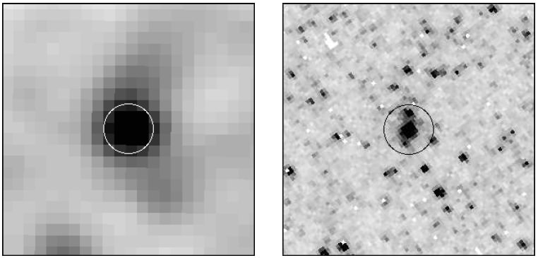
Incidentally, unaccounted for light from unresolved stars isn’t merely a problem for exoplanet studies. The issue is rather pertinent when researching the cosmic distance scale and the Hubble constant (expansion rate of the Universe). Consider the images above which feature the same field in M33. The image exhibited on the left is from a ground-based facility, whereas the higher-resolution image displayed on the right is from the Hubble Space Telescope (HST). The brightest star at the center of the image is a Cepheid variable star, which is a pulsating star that is used to establish distances to galaxies. In turn those distances are subsequently employed to determine the Hubble constant. The HST image reveals stars that are unresolved in the ground-based image, and thus the distance inferred from that observation is compromised since the Cepheid appears (spuriously) brighter than it should be.

“Blending [e.g., added light caused by unresolved stars] leads to systematically low distances to galaxies observed with the HST, and therefore to systematically high estimates of the Hubble constant,” remarked Mochejska et al. 2004. However, there is an ongoing debate concerning the importance of such an effect (Ferrarese et al. 2000, Mochejska et al. 2001).

In sum, numerous groups are developing methods to identify pseudo-planets in the Kepler database. Given the large sample and sizable investment of time required to confirm a planet candidate: such efforts are important (e.g., Bryson et al. 2013). Data from the Kepler mission have helped advance our understanding of stars and their orbiting planets, and more is yet to come. If you’d like to help the Kepler team identify planets around other stars: join the Planet Hunters citizen science project.

The Bryson et al. 2013 findings have been submitted to PASP for peer review, and a preprint is available on arXiv. The coauthors on the study are J. Jenkins, R. Gilliland, J. Twicken, B. Clarke, J. Rowe, D. Caldwell, N. Batalha, F. Mullally, M. Haas, and P. Tenenbaum. The interested reader desiring additional information will find the following pertinent: Adams et al. 2012, Collier Cameron 2012 (e.g., for other scenarios that can mimic the lightcurve of a transiting-planet), “Strange New Worlds: The Search for Alien Planets and Life beyond Our Solar System” by Ray Jayawardhana, “Distant Wanderers: The Search for Planets Beyond the Solar System” by Bruce Dorminey. For discussion on how light from unresolved sources affects the cosmic distance scale see Mochejska et al. 2004 (and for the opposite point of view, and subsequent rebuttal: Ferrarese et al. 2000, Mochejska et al. 2001).

March 16, 2013December 23, 2015 by Elizabeth Howell

Survival: Terrifying Moments in Space Flight

Apollo 13's dangerous explosion in 1970 inspired a movie, released in 1995, that starred (left to right) Bill Paxton, Kevin Bacon and Tom Hanks. Credit: Universal Pictures

Space is a dangerous and sometimes fatal business, but happily there were moments where a situation happened and the astronauts were able to recover.

An example: today (March 16) in 1966, Neil Armstrong and Dave Scott were just starting the Gemini 8 mission. They latched on to an Agena target in the hopes of doing some docking maneuvers. Then the spacecraft started spinning inexplicably.

They undocked and found themselves tumbling once per second while still out of reach of ground stations. A thruster was stuck open. Quick-thinking Armstrong engaged the landing system and stabilized the spacecraft. This cut the mission short, but saved the astronauts’ lives.

Gemini 8's Agena target before a stuck thruster on the spacecraft put the astronauts in a terrifying tumble. Credit: NASA — Gemini 8’s Agena target before a stuck thruster on the spacecraft put the astronauts in a terrifying tumble. Credit: NASA

Here are some other scary moments that astronauts in space faced, and survived:

Friendship 7: False landing bag indicator (1962)

Astronaut John Glenn views stencilling used as a model to paint the words "Friendship 7" on his spacecraft. Credit: NASA — Astronaut John Glenn views stencilling used as a model to paint the words “Friendship 7” on his spacecraft. Credit: NASA

John Glenn was only the third American in space, so you can imagine the amount of media attention he received during his three-orbit flight. NASA received an indication that his landing bag had deployed while he was still in space. Friendship 7’s Mercury spacecraft had its landing cushion underneath the heat shield, so NASA feared it had ripped away. Officials eventually informed Glenn to keep his retrorocket package strapped to the spacecraft during re-entry, rather than jettisoning it, in the hopes the package would keep the heat shield on. Glenn arrived home safely. It turned out to be a false indicator.

Apollo 11: Empty fuel tank (1969)

Apollo 11's Eagle spacecraft, as seen from fellow spaceship Columbia. Credit: NASA — Apollo 11’s Eagle spacecraft, as seen from fellow spaceship Columbia. Credit: NASA

Shortly after Neil Armstrong announced “Houston, Tranquility Base, here, the Eagle has landed” during Apollo 11, capsule communicator Charlie Duke answered, “Roger, Tranquility. We copy you on the ground. You got a bunch of guys about to turn blue. We’re breathing again. Thanks a lot.” They weren’t holding their breath just because it was the first landing on the moon; Armstrong was navigating a spacecraft that was almost out of fuel. The spacecraft Eagle overshot its landing and Armstrong did a series of maneuvers to put it on relatively flat ground. Accounts say he had less than 30 seconds of fuel when he landed on July 20, 1969.

Apollo 12: Lightning strike (1969)

Apollo 12's launch in 1969, moments before the rocket was struck by lightning. Credit: NASA — Apollo 12’s launch in 1969, moments before the rocket was struck by lightning. Credit: NASA

Moments after Apollo 12 headed from ground towards orbit, a lightning bolt hit the rocket and caused the spacecraft to go into what appeared to be a sort of zombie mode. The rocket was still flying, but the astronauts (and people on the ground) were unsure what to do. Scrambling, one controller suggested a command that essentially reset the spacecraft, and Apollo 12 was on its way. NASA did take some time to do some double-checking in orbit, to be sure, before carrying on with the rest of the mission. The agency also changed procedures about launching in stormy weather.

Apollo 13: Oxygen tank explosion (1970)

Evidence of the Apollo 13 explosion on the spacecraft Odyssey. Credit: NASA — Evidence of the Apollo 13 explosion on the service module. Credit: NASA

The astronauts of Apollo 13 performed a routine stir of the oxygen tanks on April 13, 1970. That’s when they felt the spacecraft shudder around them, and warning lights lit up. It turned out that an oxygen tank, damaged through a series of ground errors, had exploded in the service module that fed the spacecraft Odyssey, damaging some of its systems. The astronauts survived for days on minimal power in Aquarius, the healthy lunar module that was originally supposed to land on the moon. They arrived home exhausted and cold, but very much alive.

Apollo-Soyuz Test Project: Toxic vapours during landing (1975)

The Apollo command module used in the Apollo-Soyuz Test Project, during recovery. Credit: NASA

The Apollo-Soyuz Test Project was supposed to test out how well American and Russian systems (and people) would work together in space. Using an Apollo command module and a Russian Soyuz, astronauts and cosmonauts met in orbit and marked the first mission between the two nations. That almost ended in tragedy when the Americans returned to Earth and their spacecraft was inadvertently flooded with vapours from the thruster fuel. “I started to grunt-breathe to make sure I got pressure in my lungs to keep my head clear. I looked over at Vance [Brand] and he was just hanging in his straps. He was unconscious,” recalled commander Deke Slayton, in a NASA history book about the event. Slayton ensured the entire crew had oxygen masks, Brand revived quickly, and the mission ended shortly afterwards.

Mir: The fire (1997)

Jerry Linenger dons a mask during his mission on Mir in 1997. Credit: NASA

The crew on Mir was igniting a perchlorate canister for supplemental oxygen when it unexpectedly ignited. As they scrambled to put out the fire, NASA astronaut Jerry Linenger discovered at least one oxygen mask on board were malfunctioning as well. The crew managed to contain the fire quickly. Even though it affected life aboard the station for a while afterwards, the crew survived, did not need to evacuate, and helped NASA learn lessons that they still use aboard the International Space Station today.

STS-51F: Abort to orbit (1985)

STS-51F aborted to orbit during its launch. Credit: NASA

The crew of space shuttle Challenger endured two aborts on this mission. The first one took place at T-3 seconds on July 12, when a coolant valve in one of the shuttle’s engines malfunctioned. NASA fixed the problem, only to face another abort situation shortly after liftoff on July 29. One of the engines shut down too early, forcing the crew to abort to orbit. The crew was able to carry on its mission, however, including many science experiments aboard Spacelab.

STS-114: Foam hitting Discovery (2005)

Discovery during STS-114, as seen from the International Space Station. CREDIT: NASA

When Discovery lifted off in 2005, the fate of the entire shuttle program was resting upon its shoulders. NASA had implemented a series of fixes after the Columbia disaster of 2003, including redesigning the process that led to foam shedding off Columbia’s external tank and breaching the shuttle wing. Wayne Hale, a senior official in the shuttle program, later recalled his terror when he heard of more foam loss on Discovery: “I think that must have been the worst call of my life. Once earlier I had gotten a call that my child had been in an auto accident and was being taken to the hospital in an ambulance. That was a bad call. This was worse.” The foam, thankfully, struck nothing crucial and the crew survived. NASA later discovered the cracks in the foam are linked to changes in temperature the tank undergoes, and made more changes in time for a much more successful mission in 2006.

We’ve probably missed some scary moments in space, so which ones do you recall?

March 16, 2013December 30, 2015 by Nancy Atkinson

Expedition 34 Crew Gets a Foggy Welcome Home

Three members of the Expedition 34 crew undocked from the International Space Station a day later than originally planned on Friday due to bad weather in the landing area in Kazakhstan, but returned safely to Earth, despite continuing cold, foggy weather. The deteriorating weather conditions allowed only two of 12 search and rescue helicopters to land at the touchdown site because of heavy clouds and fog. NASA TV was unable to show the actual landing after the Soyuz capsule descended into the dense fog.
Continue reading “Expedition 34 Crew Gets a Foggy Welcome Home”

March 15, 2013December 23, 2015 by Jason Major

What Mount Sharp Would Look Like on Earth

Gale crater's central peak as it might look under Earthly lighting (NASA/JPL-Caltech/MSSS)

Ahh — there’s nothing like a beautiful sunny day in Gale crater! The rusty sand crunching beneath your wheels, a gentle breeze blowing at a balmy 6º C (43º F), Mount Sharp rising in the distance into a clear blue sky… wait, did I just say blue sky?

I sure did. But no worries — Mars hasn’t sprouted a nitrogen-and-oxygen atmosphere overnight. The image above is a crop from a panoramic mosaic made of images from NASA’s Curiosity rover, showing Gale crater’s central peak Mount Sharp (or Aeolis Mons, if you prefer the official moniker.) Don’t let the blue sky fool you though — the lighting has been adjusted to look like a sunlit scene on Earth, if only to let geologists more easily refer to their own experience when studying the Martian landscape.

Click the image to see the full panorama, and a view of the same scene under more “natural” Martian lighting can be found below:

Aeolis Mons panorama seen in natural lighting (NASA/JPL-Caltech/MSSS)

According to JPL, in both versions the sky has been filled out by extrapolating color and brightness information from the portions of the sky that were captured in images of the terrain.

The elevation of Mt. Sharp compared to three mountains on Earth (NASA/JPL-Caltech/MSSS)

The component images were taken by the 100-millimeter-focal-length telephoto lens camera mounted on the right side of Curiosity’s remote sensing mast, during the 45th Martian day of the rover’s mission on Mars (Sept. 20, 2012).

Informally named after planetary scientist Robert Sharp by the MSL science team, the peak rises rises more than 3 miles (5 kilometers) above the floor of Gale crater.

See more news and images from the Curiosity rover here (and to find out what the latest weather conditions in Gale crater are visit MarsWeather.com here.)

March 15, 2013December 23, 2015 by Nancy Atkinson

Could There be 100 Billion Potentially Habitable Planets in the Galaxy?

A visualization of the “unseen” red dwarfs in the night sky. Credit: D. Aguilar & C. Pulliam (CfA)

As we’ve reported recently, the likelihood of findings habitable Earth-sized worlds just seems to keep getting better and better. But now the latest calculations from a new paper out this week are almost mind-bending. Using what the authors call a “very careful extrapolation” of the rate of small planets observed around M dwarf stars by the Kepler spacecraft, they estimate there could be upwards of 100 billion Earth-sized worlds in the habitable zones of M dwarf or red dwarf stars in our galaxy. And since the population of these stars themselves are estimated to be around 100 billion in the Milky Way, that’s – on average – an Earth-sized world for every red dwarf star in our galaxy.

Whoa.

And since our solar system is surrounded by red dwarfs – very cool, very dim stars not visible to the naked eye (less than a thousandth the brightness of the Sun) — these worlds could be close by, perhaps as close as 7 light-years away.

With the help of astronomer Darin Ragozzine, a postdoctoral associate at the University of Florida who works with the Kepler mission (see our Hangout interview with him last year), let’s take a look back at the recent findings that brought about this latest stunning projection.

Back in February, we reported on the findings from Courtney Dressing and Dave Charbonneau from the Center for Astrophysics that said about 6% of red dwarf stars could host Earth-size habitable planets. But since then, Dressing and Charbonneau realized they had a bug in their code and they have revised the frequency to 15%, not 6%. That more than doubles the estimates.

Then, just this week we reported how Ravi Kopparapu from at Penn State University and the Virtual Planetary Lab at University of Washington suggested that the habitable zone around planets should be redefined, based on new, more precise data that puts the habitable zones farther away from the stars than previously thought. Applying the new habitable zone to red dwarfs pushes the fraction of red dwarfs having habitable planets closer to 50%.

The graphic shows optimistic and conservative habitable zone boundaries around cool, low mass stars. The numbers indicate the names of known Kepler planet candidates. Yellow color represents candidates with less than 1.4 times Earth-radius. Green color represents planet candidates between 1.4 and 2 Earth radius. Credit: Penn State.

But now, the new paper submitted to arXiv this week, “The Radius Distribution of Small Planets Around Cool Stars” by Tim Morton and Jonathan Swift (a grad student and postdoc from Caltech’s ExoLab) finds there is an additional correction to the numbers by Dressing and Charbonneau numbers.

“This is basically due to the fact that there are more small planets than we thought because Kepler isn’t yet sensitive to a large number that take longer to orbit,” Ragozzine told Universe Today. “Accounting for this effect and enhancing the calculation using some nice new statistical techniques, they estimate that the Dressing and Charbonneau numbers are actually too small by a factor of 2. This puts the number at 30% in the old habitable zone, and now up to about 100% in the new habitable zone.”

Now, it is important to point out a few things about this.

As Morton noted in an email to Universe Today, it’s important to realize that this is not yet a direct measurement of the habitable zone rate, “but it is what I would classify as a very careful extrapolation of the rate of small planets we have observed at shorter periods around M dwarfs.”

And as Ragozzine and Morton confirmed for us, all of these numbers are based on Kepler results only, and so far, while there confirmed planets around M dwarfs, there are none confirmed so far in the habitable zone.

“They do not use any results from Radial Velocity (HARPS, etc.),” Ragozzine said. “As such, these are all candidates and not planets. That is, the numbers are based on an assumption that most/all of the Kepler candidates are true planets. There are varying opinions about what the false positive rate would be, especially for this particular subset of stars, but there’s no question that the numbers may go down because some of these candidates turn out to be something else other than HZ Earth-size planets.”

Other caveats need to be considered, as well.

“Everyone needs to be careful about what “100%” means,” Ragozzine said. “It does not mean that every M dwarf has a HZ Earth-size planet. It means that, on average, there is 1 HZ-Earth size planet for every M dwarf. The difference comes from the fact that these small stars tend to have planets that come in packs of 3-5. If, on average, the number of planets per star is one, and the typical M star has 5 planets, then only 20% of M stars have planetary systems.”

The point is subtle but important. For example, if you want to plan new telescope missions to observe these planets, understanding their distribution is critical, Ragozzine said.

“I’m very interested in understanding what kinds of planetary systems host these planets as this opens a number of interesting scientific questions. Discerning their frequency and distribution are both valuable.”

Additionally, the new definition of the habitable zone from Kopparapu et al. makes a big difference.

As Ragozzine points out:

“This is really starting to point out that the definition of the HZ is based on mostly theoretical arguments that are hard to rigorously justify,” Ragozzine said. “For example, a recent paper came out showing that atmospheric pressure makes a big difference but there’s no way to estimate what the pressure will be on a distant world. (Even in the best cases, we can barely tell that the whole planet isn’t one giant puffy atmosphere.) Work by Kopparapu and others is clearly necessary and, from an astrobiological point of view, we have no choice but to use the best theory and assumptions available. Still, some of us in the field are starting to become really wary of the “H-word” (as Mike Brown calls it), wondering if it is just too speculative. Incidentally, I much, much prefer that these worlds be referred to as potentially habitable, since that’s really what we’re trying to say.”

However, Morten told Universe Today that he feels the biggest difference in their work was the careful extrapolation from short period planets to longer periods. “This is why we get occurrence rates for the smaller planets that are twice as large as Dressing or Kopparapu,” he said via email.

He also thinks the most interesting thing in their paper is not just the overall occurrence rate or the HZ occurrence rate even, but the fact that, for the first time, they’ve identified some interesting structure in the distribution of exoplanet radii.

“For example, we show that it appears that planets of roughly 1 Earth radius are actually the most common size of planet around these cool stars,” Morton said. “This makes some intuitive sense given the rocky bodies in our Solar System—there are two planets about the size of Earth, making it the most common size of small planet in our system too! Also, we find that there are lots and lots of planets around M dwarfs that are just beyond the detection threshold of current ground-based transiting surveys—this means that as more sensitive instruments and surveys are designed, we will just keep finding more and more of these exciting planets!”

But Ragozzine told us that even with all aforementioned caveats, the exciting thing is that the main gist of these new numbers probably won’t change much.

“No one is expecting that the answer will be different by more than a factor of a few – i.e., the true range is almost certainly between 30-300% and very likely between 70-130%,” Ragozzine said. “As the Kepler candidate list improves in quantity (due to new data), purity, and uniformity, the main goal will be to justify these statements and to significantly reduce that range.”

Another fun aspect is that this new work is being done by the young generation of astronomers, grad students and postdocs.

“I’m sure this group and others will continue producing great things… the exciting scientific results are just beginning!” Ragozzine said.

March 15, 2013December 23, 2015 by Nancy Atkinson

ALMA: The View from a Different World

This image shows an aerial view of the Chajnantor Plateau, located at an altitude of 5000 meters in the Chilean Andes, where the array of ALMA antennas is located. Credit: Clem & Adri Bacri-Normier (wingsforscience.com)/ESO.

A new film called The View From Mars takes a look ALMA (Atacama Large Millimeter Array), the huge international telescope project that was inaugurated in Chile this week. It is located in the Atacama Desert, the driest place on Earth and an area that bears a striking resemblance to the Red Planet.

But the conditions there, with clear, dry skies, are perfect for astronomy. ALMA’s moveable group of 66 giant antennas do not detect visible light like conventional optical telescopes. Instead they work together to gather emissions from gas, dust and stars and make observations in millimeter wavelengths, using radio frequencies instead of visible light—with no need for darkness, so the stars can be studied around the clock. With these tools, astronomers will soon be able to look billions of years into the past, gazing at the formation of distant stars and galaxies.

“In doing so,” says filmmaker Jonathan de Villiers, “they’ll build a clearer picture of how our sun and our galaxy formed.”

Here is part one; you can see part 2 at this link.

The View From Mars: Part One on Nowness.com.

March 15, 2013April 26, 2016 by David Dickinson

Citizen Science, Old-School Style: The True Tale of Operation Moonwatch

An Operation Moonwatch team in action based out of Terre Haute, Indiana. (Courtesy of Keep Watching the Skies! Author Patrick McCray, used with Permission).

Amateur astronomers have done more than just watch the skies, they’ve been a national security asset. In the mid-1950’s, it was realized that the reality of the Space Age was at best only a decade away. Sub-orbital German V-2 rockets captured by the Soviets and the United States were reaching higher and higher altitudes, and it was only a matter of time before orbital velocity would be achieved.

Keep in mind, this was the age of backyard bomb shelters, “duck and cover” drills, and civil preparedness as Cold War fever reached a heightened pitch. Ground Observer Corps encouraged and trained citizen groups how to spot and report enemy bombers approaching the U.S coast in preparation for a nuclear confrontation. And remember, there was no reason to think that this build up wouldn’t extend to the militarization of space. It was in this era that Operation Moonwatch was born.

Conceived by Harvard astronomer Fred Whipple, Operation Moonwatch was the “Galaxy Zoo” of its day. The idea was simple; teams of observers around the world would track, time and record satellite passes over their location and feed this data back to the computation center at Cambridge, Massachusetts (telephone, Western Union or ham radio were the methods of the day) This data would give engineers information as to where to point their enormous Baker-Nunn cameras. These instruments were wide-field Schmidt cameras that could cover large swaths of the sky. They were to be positioned at 12 locations worldwide to keep tabs on satellites in low Earth orbit (LEO).

A Baker-Nunn satellite tracking camera ready for action. (Credit: NASA).

To be sure, there were obstacles to overcome. The Baker-Nunn cameras were well behind schedule, and the entire system was struggling to come online by mid-1958 in time for the International Geophysical Year (IGY). School and community groups had to be organized, trained, and equipped. Knowing precise location in the pre-GPS era had to be addressed. Many purchased optical kits available from Radio Shack, while many teams built their own. Then there was the dilemma of what a satellite would actually look like to an observer on the ground. Could a trained spotter even see it? Civil Air Patrol groups experimented with various trial substitutions, such as following aircraft, flocks of birds and bats at dusk and even tracking pebbles tossed into the sky!

Operation Moonwatch was also to play a part of the 1958 International Geophysical Year. Many doubted to effectiveness of amateur groups, but public interest ran high. Then on October 4th 1957, the world was caught off guard as Sputnik 1 lifted off from the Baikonur Cosmodrome.

The metal ball that started it all... Sputnik 1. (Credit: NASA/Asif A. Siddiqi). — The metal ball that started it all… Sputnik 1. (Credit: NASA/Asif A. Siddiqi).

The world was stunned that the Soviets had beaten the West into space. The National Advisory Committee for Aeronautics (later to become NASA in 1958) had yet to achieve a successful orbital launch, and the United States Naval Research Laboratory was still floundering to get the Vanguard program off the pad. The launch of Sputnik found a scant few Moonwatch teams at the ready to catch its first dusk passes over the United States. Keep in mind, the Sputnik satellite was too small and faint to see with the naked eye. What most casual observers in the general public saw (remember the opening scenes in the movie October Sky?) was actually the rocket booster that put Sputnik into space.

Moonwatch teams would “look up by looking down” using a bench mounted telescope that looked at a reflective plate aimed skyward. With observers arranged in a row aimed at a picket line, they would call out when the target satellite crossed the local meridian. This would in turn be documented by an onsite recorder for transmission.

A classic Operation Moonwatch bench instrument sold by Edmund Scientifc. (Credit: The Smithsonian Natinal Air & Space Museum). — A classic Operation Moonwatch bench instrument sold by Edmund Scientific (Credit: The Smithsonian National Air & Space Museum).

With Sputnik, the Operation Moonwatch volunteers found themselves thrust into the spotlight. Newspapers & radio shows clamored to interview volunteers, as the public suddenly became obsessed with space. Moonwatchers followed and documented to launch of the dog Laika aboard Sputnik 2 on November 3^rd, 1957, and when the U.S. finally launched its first satellite Explorer I on February 1^st 1958 Operation Moonwatch tracked it. Magazines such as National Geographic and Boys Life ran articles on the project and told teams how they could participate. When Sputnik 4 reentered over the U.S. on September 1962, it was data from Operation Moonwatch observers that proved vital in its recovery.

How Operation Moonwatch fit into the hierarchy. (Credit: NASA archives, The Role of the NAS & TPESP). — How Operation Moonwatch fit into the hierarchy. Note how amateur groups were associated with this press. (Credit: NASA archives, *The Role of the NAS & TPESP*).

Moonwatch was disbanded in 1975, but many volunteers continued tracking satellites and sharing data on their own. I always think that it’s fascinating that three very early satellites from the early days of Operation Moonwatch are still in orbit and can been seen with a good pair of binoculars and a little patience , Vanguards 1, 2 & 3. It could be argued that Operation Moonwatch provided a civilian means to monitor the goings on of governments in low Earth orbit and may have contributed to the Outer Space Treaty outlawing the use of nuclear weapons in space. Another fortunate occurrence of the era was the establishment of a civilian space agency in the U.S., argued for successfully by Dr. James Van Allen. How different would the course of history have been if the U.S. space program had become a “fourth branch” of the military?

Cincinnati plaque commemorating Operation Moonwatch. (Brian Van Flandern Public Domain image).

Today, modern satellite trackers still follow, image and share information on satellites worldwide. This effort transcends borders; when hazardous payloads such as Russia’s failed Mars mission Phobos-Grunt reentered in early 2012 satellite trackers documented its final passage, and efforts are still underway to keep tabs on the USAF’s X-37 spy satellite. One can also see a stark contrast between the efforts to enlist civilian effort during the Cold War and the modern Global War on Terrorism. Interest in science was at an all-time high in the 1950’s, as it was realized the West might be lagging behind in science education. In a post-9/11 era, there almost seems to be a movement to isolate participation. Many model rocketry groups are under increased restriction, and even amateur astronomers may see essential tools such as green laser pointers restricted for use.

Image of Space Shuttle Discovery on STS-119 captured from the ground… note the NASA “Blue Meatball” logo on the wing! (Credit: Ralf Vandebergh, used with permission).

But the good news is, anyone can still track a satellite from the comfort of their own backyard all in the spirit of Operation Moonwatch. DARPA announced a project last year which may resurrect a program similar to Operation Moonwatch. Named SpaceView, this program seeks to augment the U.S. Air Force’s Space Surveillance Network. Keep an eye on the sky, and remember a dedicated few amateur observers that played a crucial role in modern history as you watch satellites drift silently by in the twilight skies.

For more on the fscinating hostory of Operation Moonwatch, read Patrick McCray’s Keep Watching the Skies!

See more of Ralf Vandebergh’s outstanding work at his site Telescopic Spaceflight Images.

March 15, 2013April 8, 2018 by Nancy Atkinson

Astrophotos: Latest Images and Videos of Comet PANSTARRS

C/2011 L4 (PANSTARRS on March 15, 2013. Taken in Hachimantai City Japan. Credit and copyright: Jason Hill.

You want images and videos of Comet C/2011 L4 (PANSTARRS)? We’ve got ’em! We’ll start with this stunning view from Japan, taken by Jason Hill. But there’s lots more below:

A first capture of Comet PANSTARRS on March 14, 2013. Credit and copyright: Adam Wipp.

Another first view of Comet PANSTARRS from Valencia, Spain on March 14, 2013. Credit and copyright: Alejandro Garcia.

This timelapse comes from Andrew Takano, a graduate student at the University of Texas at Austin:

Another great timelapse comes from a public observaing event in Greece, sent to us by J.D Strikis and the Hellenic Amateur Astronomy Association:

Comet PanStarrs C/2012 L4 Public Observing in Greece from J.D.Strikis on Vimeo.

Comet PANSTARRS on March 14, 2013, as seen in the Arizona skies. Credit and copyright: Chris Schur.

Photographer Chris Schur said last night’s views were “the best and brightest comet yet in the western Arizona Sunset sky!” Schur said via email. “I was able to go much deeper tonight using an 80mm Zeiss refractor and Canon Xti. The head shows more fan like protrusions, and the tail is now really shaping up. … The comet here at our elevation of 5150 feet was very easy to see the entire time it was up, and I would rate it at first magnitude for sure.”

Comet PANSTARRS as seen from Aarhus, Denmark (56.2 N, 10.2 E). Credit and copyright: Jens Riggelsen.

Comet Panstarrs above Boulder, Colorado on the evening of March 13, 2013, courtesy of Patrick Cullis:

Comet PANSTARRS on March 13, 2013 as see from Newington, New Hampshire, USA. Credit and copyright: John Gianforte (theskyguy.org)

Comet PANSTARRS seen from Oakland, California. The Port of Oakland and the Bay Bridge are in the foreground with the comet and crescent moon in the background. Taken on March 12, 2013. Credit and copyright: Jared Wilson.

Comet C/2011 L4 (PANSTARRS) floats in the twilight sky over the lighthouses and pier at Grand Haven State Park in Grand Haven, Michigan on March 13, 2013. Credit and copyright: Kevin's Stuff on Flickr. — Comet C/2011 L4 (PANSTARRS) floats in the twilight sky over the lighthouses and pier at Grand Haven State Park in Grand Haven, Michigan on March 13, 2013. Credit and copyright: Kevin’s Stuff on Flickr.

Comet PANSTARRS and a 5% illuminated Moon on March 13, 2013. Credit and copyright: Tavi Greiner.

You can see more at our Flickr page, and we’ll keep adding and posting! Thanks to everyone who has been so generous with sharing their great photos and videos.

Want to get your astrophoto featured on Universe Today? Join our Flickr group or send us your images by email (this means you’re giving us permission to post them). Please explain what’s in the picture, when you took it, the equipment you used, etc.

March 15, 2013December 23, 2015 by Nancy Atkinson

Watch Live Webcast of Comet PANSTARRS

UPDATE: The webcast has been moved to March 16 at 17:00 UTC (1 pm EDT) due to bad weather in Italy.

Has it been cloudy where you live and you haven’t yet been able to see Comet PANSTARRS? The Virtual Telescope Project will have a live webcast of this comet, C/2011 L4 PANSTARRS, from Italy, ~~March 15~~, on March 16 at 17:00 UTC, 1 p.m. EDT. “We have been waiting for it for over one year, and now the waiting is over,” said astrophysicist Gianluca Masi, who will host the webcast, which you can see at this link. Masi said they are keeping an eye on the skies, and will keep us updated on if they need to change the time of the webcast.

If you’re waiting for the weekend to see it with your own eyes, check out our detailed guides on how to see it here and here. Both are filled with graphics and great info on how to see this comet.

This comet has been a challenge to see, and was actually closest to the Sun on March 10, meaning that is when it was at its brightest. However, while Comet PANSTARRS will fade over the next few weeks, it will also rise higher into a darker sky and become – for a time – easier to see. So keep looking!

March 15, 2013December 23, 2015 by Elizabeth Howell

Why You’ll Never See a Red Comet Like in ‘Game of Thrones’

That red comet is pretty, but perhaps not so realistic. Credit: Game of Thrones Wiki/HBO (Screencap)

A blood-red comet appears in the sky. People quake in its wake.

This phenomenon, which happens in the second season of the medieval fantasy Game of Thrones, had us all wondering — can you ever actually see a red comet?

We talked to Matthew Knight, an astronomer at the Lowell Observatory in Arizona who observes comets. He gave us some answers just in time for the third season of Game of Thrones, which begins March 31.

At first blush, he said, the comet’s red color wouldn’t be possible because the strongest emissions from comets are in the blue and green regions, mostly from neutral gases such as hydroxide and cyanide.

There is a type of emission that is close to red, called “forbidden oxygen”, which occurs when atoms make a rare energy transition between states of “excitement”. But it’s very faint and short-lived, Knight wrote.

The visible light from a comet comes from a combination of reflected solar continuum (sunlight reflecting off of dust grains) and cometary emission (neutral and/or ionized molecules of gas that emit photons at a particular wavelength). The sunlight reflecting off of dust grains basically looks like sunlight and since the Sun appears yellow/white, this component cannot look red.

A small caveat is that due to the physical properties of dust grains, comet dust often actually does “redden” sunlight slightly when measured with sensitive equipment. However, this reddening is at a very low level and is not enough to cause the reflected sunlight to appear a deep red like in Game of Thrones. The strongest comet emissions in the region where human eyes can see are in the blue and green regions.

Comet Hale-Bopp. which displays the usual cometary colors. Credit: E. Kolmhofer, H. Raab; Johannes-Kepler-Observatory, Linz, Austria

So what ingredients does a comet need to look like the one in Game of Thrones? According to Knight, it would have to meet these criteria:

Be visible in daylight, which really only happens about once a century;
Be close to the sun (he supposes this one is, given how straight the tail is);
Have a “strange composition” that is different from anything we know in the solar system. The composition could be that forbidden oxygen he talked about, coming from a comet whose ices are carbon monoxide and carbon dioxide. But that would be hard, because those types of ices would not survive long when exposed to sunlight.

If we really want to think in a science fiction vein, Knight suggests that maybe the comet could be made up unpredictably:

Alternatively it could be something else entirely unknown in cometary chemistry or dust, with really weird properties causing a much stronger reddening than is normally seen. In any event, the composition would be so anomalous that this comet would almost certainly have originated in another solar system. That would make comet scientists very interested in studying it!

But don’t despair yet. Comet ISON might be bright enough for daylight viewing when it swings by Earth late in 2013. Comets are unpredictable beasts, but we’re pretty sure of one thing: no matter how bright it is, it won’t look red.