Gale crater's central peak as it might look under Earthly lighting (NASA/JPL-Caltech/MSSS)
Ahh — there’s nothing like a beautiful sunny day in Gale crater! The rusty sand crunching beneath your wheels, a gentle breeze blowing at a balmy 6º C (43º F), Mount Sharp rising in the distance into a clear blue sky… wait, did I just say blue sky?
I sure did. But no worries — Mars hasn’t sprouted a nitrogen-and-oxygen atmosphere overnight. The image above is a crop from a panoramic mosaic made of images from NASA’s Curiosity rover, showing Gale crater’s central peak Mount Sharp (or Aeolis Mons, if you prefer the official moniker.) Don’t let the blue sky fool you though — the lighting has been adjusted to look like a sunlit scene on Earth, if only to let geologists more easily refer to their own experience when studying the Martian landscape.
Click the image to see the full panorama, and a view of the same scene under more “natural” Martian lighting can be found below:
Aeolis Mons panorama seen in natural lighting (NASA/JPL-Caltech/MSSS)
According to JPL, in both versions the sky has been filled out by extrapolating color and brightness information from the portions of the sky that were captured in images of the terrain.
The elevation of Mt. Sharp compared to three mountains on Earth (NASA/JPL-Caltech/MSSS)
The component images were taken by the 100-millimeter-focal-length telephoto lens camera mounted on the right side of Curiosity’s remote sensing mast, during the 45th Martian day of the rover’s mission on Mars (Sept. 20, 2012).
Informally named after planetary scientist Robert Sharp by the MSL science team, the peak rises rises more than 3 miles (5 kilometers) above the floor of Gale crater.
See more news and images from the Curiosity rover here (and to find out what the latest weather conditions in Gale crater are visit MarsWeather.com here.)
A visualization of the “unseen” red dwarfs in the night sky. Credit: D. Aguilar & C. Pulliam (CfA)
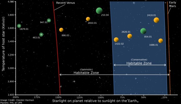
As we’ve reported recently, the likelihood of findings habitable Earth-sized worlds just seems to keep getting better and better. But now the latest calculations from a new paper out this week are almost mind-bending. Using what the authors call a “very careful extrapolation” of the rate of small planets observed around M dwarf stars by the Kepler spacecraft, they estimate there could be upwards of 100 billion Earth-sized worlds in the habitable zones of M dwarf or red dwarf stars in our galaxy. And since the population of these stars themselves are estimated to be around 100 billion in the Milky Way, that’s – on average – an Earth-sized world for every red dwarf star in our galaxy.
Whoa.
And since our solar system is surrounded by red dwarfs – very cool, very dim stars not visible to the naked eye (less than a thousandth the brightness of the Sun) — these worlds could be close by, perhaps as close as 7 light-years away.
With the help of astronomer Darin Ragozzine, a postdoctoral associate at the University of Florida who works with the Kepler mission (see our Hangout interview with him last year), let’s take a look back at the recent findings that brought about this latest stunning projection.
Back in February, we reported on the findings from Courtney Dressing and Dave Charbonneau from the Center for Astrophysics that said about 6% of red dwarf stars could host Earth-size habitable planets. But since then, Dressing and Charbonneau realized they had a bug in their code and they have revised the frequency to 15%, not 6%. That more than doubles the estimates.
Then, just this week we reported how Ravi Kopparapu from at Penn State University and the Virtual Planetary Lab at University of Washington suggested that the habitable zone around planets should be redefined, based on new, more precise data that puts the habitable zones farther away from the stars than previously thought. Applying the new habitable zone to red dwarfs pushes the fraction of red dwarfs having habitable planets closer to 50%.
The graphic shows optimistic and conservative habitable zone boundaries around cool, low mass stars. The numbers indicate the names of known Kepler planet candidates. Yellow color represents candidates with less than 1.4 times Earth-radius. Green color represents planet candidates between 1.4 and 2 Earth radius. Credit: Penn State.
But now, the new paper submitted to arXiv this week, “The Radius Distribution of Small Planets Around Cool Stars” by Tim Morton and Jonathan Swift (a grad student and postdoc from Caltech’s ExoLab) finds there is an additional correction to the numbers by Dressing and Charbonneau numbers.
“This is basically due to the fact that there are more small planets than we thought because Kepler isn’t yet sensitive to a large number that take longer to orbit,” Ragozzine told Universe Today. “Accounting for this effect and enhancing the calculation using some nice new statistical techniques, they estimate that the Dressing and Charbonneau numbers are actually too small by a factor of 2. This puts the number at 30% in the old habitable zone, and now up to about 100% in the new habitable zone.”
Now, it is important to point out a few things about this.
As Morton noted in an email to Universe Today, it’s important to realize that this is not yet a direct measurement of the habitable zone rate, “but it is what I would classify as a very careful extrapolation of the rate of small planets we have observed at shorter periods around M dwarfs.”
And as Ragozzine and Morton confirmed for us, all of these numbers are based on Kepler results only, and so far, while there confirmed planets around M dwarfs, there are none confirmed so far in the habitable zone.
“They do not use any results from Radial Velocity (HARPS, etc.),” Ragozzine said. “As such, these are all candidates and not planets. That is, the numbers are based on an assumption that most/all of the Kepler candidates are true planets. There are varying opinions about what the false positive rate would be, especially for this particular subset of stars, but there’s no question that the numbers may go down because some of these candidates turn out to be something else other than HZ Earth-size planets.”
Other caveats need to be considered, as well.
“Everyone needs to be careful about what “100%” means,” Ragozzine said. “It does not mean that every M dwarf has a HZ Earth-size planet. It means that, on average, there is 1 HZ-Earth size planet for every M dwarf. The difference comes from the fact that these small stars tend to have planets that come in packs of 3-5. If, on average, the number of planets per star is one, and the typical M star has 5 planets, then only 20% of M stars have planetary systems.”
The point is subtle but important. For example, if you want to plan new telescope missions to observe these planets, understanding their distribution is critical, Ragozzine said.
“I’m very interested in understanding what kinds of planetary systems host these planets as this opens a number of interesting scientific questions. Discerning their frequency and distribution are both valuable.”
Additionally, the new definition of the habitable zone from Kopparapu et al. makes a big difference.
As Ragozzine points out:
“This is really starting to point out that the definition of the HZ is based on mostly theoretical arguments that are hard to rigorously justify,” Ragozzine said. “For example, a recent paper came out showing that atmospheric pressure makes a big difference but there’s no way to estimate what the pressure will be on a distant world. (Even in the best cases, we can barely tell that the whole planet isn’t one giant puffy atmosphere.) Work by Kopparapu and others is clearly necessary and, from an astrobiological point of view, we have no choice but to use the best theory and assumptions available. Still, some of us in the field are starting to become really wary of the “H-word” (as Mike Brown calls it), wondering if it is just too speculative. Incidentally, I much, much prefer that these worlds be referred to as potentially habitable, since that’s really what we’re trying to say.”
However, Morten told Universe Today that he feels the biggest difference in their work was the careful extrapolation from short period planets to longer periods. “This is why we get occurrence rates for the smaller planets that are twice as large as Dressing or Kopparapu,” he said via email.
He also thinks the most interesting thing in their paper is not just the overall occurrence rate or the HZ occurrence rate even, but the fact that, for the first time, they’ve identified some interesting structure in the distribution of exoplanet radii.
“For example, we show that it appears that planets of roughly 1 Earth radius are actually the most common size of planet around these cool stars,” Morton said. “This makes some intuitive sense given the rocky bodies in our Solar System—there are two planets about the size of Earth, making it the most common size of small planet in our system too! Also, we find that there are lots and lots of planets around M dwarfs that are just beyond the detection threshold of current ground-based transiting surveys—this means that as more sensitive instruments and surveys are designed, we will just keep finding more and more of these exciting planets!”
But Ragozzine told us that even with all aforementioned caveats, the exciting thing is that the main gist of these new numbers probably won’t change much.
“No one is expecting that the answer will be different by more than a factor of a few – i.e., the true range is almost certainly between 30-300% and very likely between 70-130%,” Ragozzine said. “As the Kepler candidate list improves in quantity (due to new data), purity, and uniformity, the main goal will be to justify these statements and to significantly reduce that range.”
Another fun aspect is that this new work is being done by the young generation of astronomers, grad students and postdocs.
“I’m sure this group and others will continue producing great things… the exciting scientific results are just beginning!” Ragozzine said.
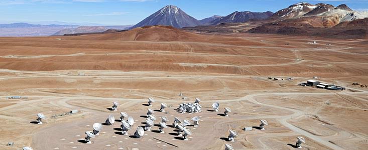
This image shows an aerial view of the Chajnantor Plateau, located at an altitude of 5000 meters in the Chilean Andes, where the array of ALMA antennas is located. Credit: Clem & Adri Bacri-Normier (wingsforscience.com)/ESO.
A new film called The View From Mars takes a look ALMA (Atacama Large Millimeter Array), the huge international telescope project that was inaugurated in Chile this week. It is located in the Atacama Desert, the driest place on Earth and an area that bears a striking resemblance to the Red Planet.
But the conditions there, with clear, dry skies, are perfect for astronomy. ALMA’s moveable group of 66 giant antennas do not detect visible light like conventional optical telescopes. Instead they work together to gather emissions from gas, dust and stars and make observations in millimeter wavelengths, using radio frequencies instead of visible light—with no need for darkness, so the stars can be studied around the clock. With these tools, astronomers will soon be able to look billions of years into the past, gazing at the formation of distant stars and galaxies.
“In doing so,” says filmmaker Jonathan de Villiers, “they’ll build a clearer picture of how our sun and our galaxy formed.”
An Operation Moonwatch team in action based out of Terre Haute, Indiana. (Courtesy of Keep Watching the Skies! Author Patrick McCray, used with Permission).
Amateur astronomers have done more than just watch the skies, they’ve been a national security asset. In the mid-1950’s, it was realized that the reality of the Space Age was at best only a decade away. Sub-orbital German V-2 rockets captured by the Soviets and the United States were reaching higher and higher altitudes, and it was only a matter of time before orbital velocity would be achieved.
Keep in mind, this was the age of backyard bomb shelters, “duck and cover” drills, and civil preparedness as Cold War fever reached a heightened pitch. Ground Observer Corps encouraged and trained citizen groups how to spot and report enemy bombers approaching the U.S coast in preparation for a nuclear confrontation. And remember, there was no reason to think that this build up wouldn’t extend to the militarization of space. It was in this era that Operation Moonwatch was born.
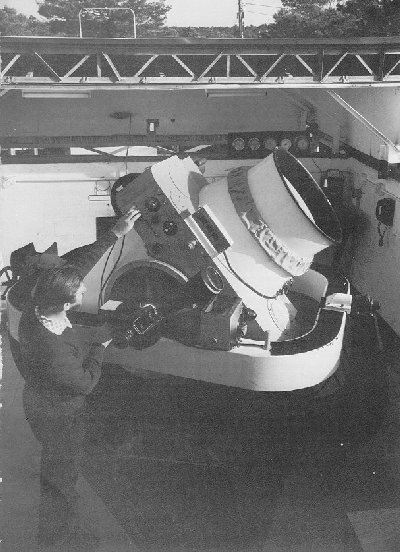
Conceived by Harvard astronomer Fred Whipple, Operation Moonwatch was the “Galaxy Zoo” of its day. The idea was simple; teams of observers around the world would track, time and record satellite passes over their location and feed this data back to the computation center at Cambridge, Massachusetts (telephone, Western Union or ham radio were the methods of the day) This data would give engineers information as to where to point their enormous Baker-Nunn cameras. These instruments were wide-field Schmidt cameras that could cover large swaths of the sky. They were to be positioned at 12 locations worldwide to keep tabs on satellites in low Earth orbit (LEO).
A Baker-Nunn satellite tracking camera ready for action. (Credit: NASA).
To be sure, there were obstacles to overcome. The Baker-Nunn cameras were well behind schedule, and the entire system was struggling to come online by mid-1958 in time for the International Geophysical Year (IGY). School and community groups had to be organized, trained, and equipped. Knowing precise location in the pre-GPS era had to be addressed. Many purchased optical kits available from Radio Shack, while many teams built their own. Then there was the dilemma of what a satellite would actually look like to an observer on the ground. Could a trained spotter even see it? Civil Air Patrol groups experimented with various trial substitutions, such as following aircraft, flocks of birds and bats at dusk and even tracking pebbles tossed into the sky!
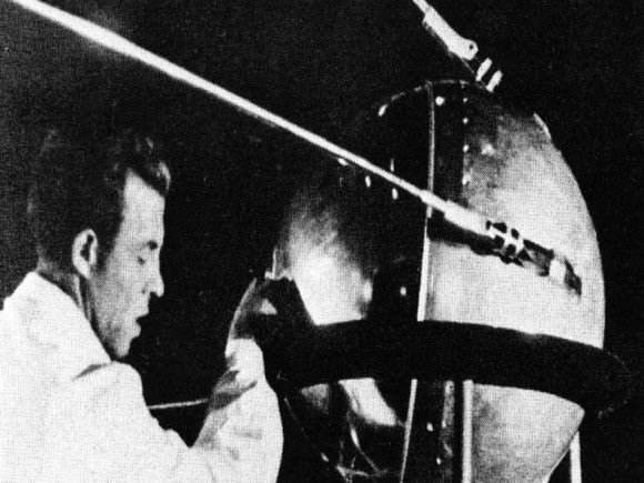
Operation Moonwatch was also to play a part of the 1958 International Geophysical Year. Many doubted to effectiveness of amateur groups, but public interest ran high. Then on October 4th 1957, the world was caught off guard as Sputnik 1 lifted off from the Baikonur Cosmodrome.
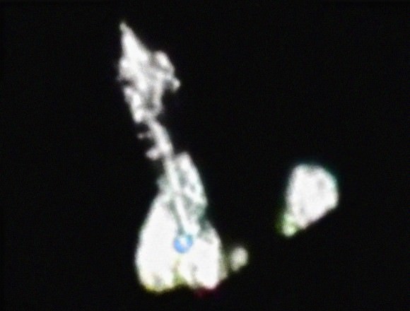
The world was stunned that the Soviets had beaten the West into space. The National Advisory Committee for Aeronautics (later to become NASA in 1958) had yet to achieve a successful orbital launch, and the United States Naval Research Laboratory was still floundering to get the Vanguard program off the pad. The launch of Sputnik found a scant few Moonwatch teams at the ready to catch its first dusk passes over the United States. Keep in mind, the Sputnik satellite was too small and faint to see with the naked eye. What most casual observers in the general public saw (remember the opening scenes in the movie October Sky?) was actually the rocket booster that put Sputnik into space.
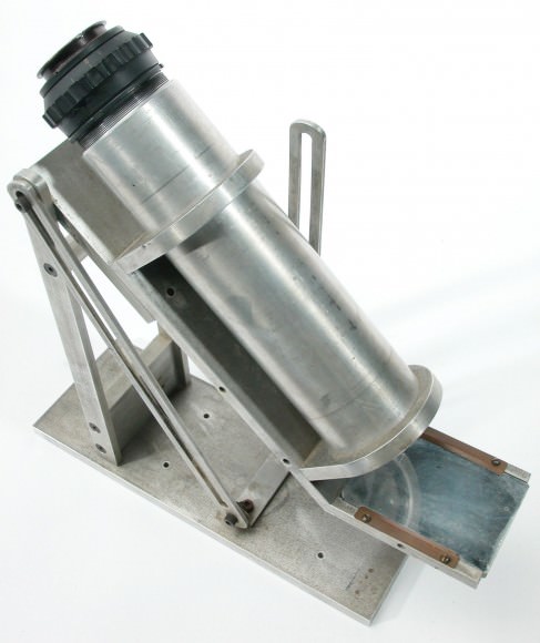
Moonwatch teams would “look up by looking down” using a bench mounted telescope that looked at a reflective plate aimed skyward. With observers arranged in a row aimed at a picket line, they would call out when the target satellite crossed the local meridian. This would in turn be documented by an onsite recorder for transmission.
With Sputnik, the Operation Moonwatch volunteers found themselves thrust into the spotlight. Newspapers & radio shows clamored to interview volunteers, as the public suddenly became obsessed with space. Moonwatchers followed and documented to launch of the dog Laika aboard Sputnik 2 on November 3rd, 1957, and when the U.S. finally launched its first satellite Explorer I on February 1st 1958 Operation Moonwatch tracked it. Magazines such as National Geographic and Boys Life ran articles on the project and told teams how they could participate. When Sputnik 4 reentered over the U.S. on September 1962, it was data from Operation Moonwatch observers that proved vital in its recovery.
How Operation Moonwatch fit into the hierarchy. Note how amateur groups were associated with this press. (Credit: NASA archives, The Role of the NAS & TPESP).
Moonwatch was disbanded in 1975, but many volunteers continued tracking satellites and sharing data on their own. I always think that it’s fascinating that three very early satellites from the early days of Operation Moonwatch are still in orbit and can been seen with a good pair of binoculars and a little patience , Vanguards 1, 2 & 3. It could be argued that Operation Moonwatch provided a civilian means to monitor the goings on of governments in low Earth orbit and may have contributed to the Outer Space Treaty outlawing the use of nuclear weapons in space. Another fortunate occurrence of the era was the establishment of a civilian space agency in the U.S., argued for successfully by Dr. James Van Allen. How different would the course of history have been if the U.S. space program had become a “fourth branch” of the military?
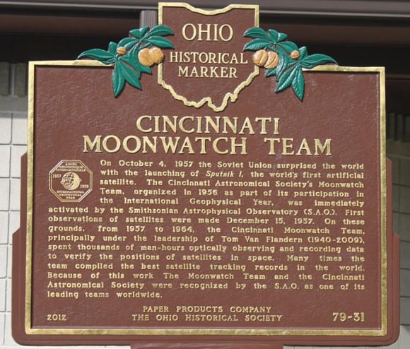
Cincinnati plaque commemorating Operation Moonwatch. (Brian Van Flandern Public Domain image).
Today, modern satellite trackers still follow, image and share information on satellites worldwide. This effort transcends borders; when hazardous payloads such as Russia’s failed Mars mission Phobos-Grunt reentered in early 2012 satellite trackers documented its final passage, and efforts are still underway to keep tabs on the USAF’s X-37 spy satellite. One can also see a stark contrast between the efforts to enlist civilian effort during the Cold War and the modern Global War on Terrorism. Interest in science was at an all-time high in the 1950’s, as it was realized the West might be lagging behind in science education. In a post-9/11 era, there almost seems to be a movement to isolate participation. Many model rocketry groups are under increased restriction, and even amateur astronomers may see essential tools such as green laser pointers restricted for use.
Image of Space Shuttle Discovery on STS-119 captured from the ground… note the NASA “Blue Meatball” logo on the wing! (Credit: Ralf Vandebergh, used with permission).
But the good news is, anyone can still track a satellite from the comfort of their own backyard all in the spirit of Operation Moonwatch. DARPA announced a project last year which may resurrect a program similar to Operation Moonwatch. Named SpaceView, this program seeks to augment the U.S. Air Force’s Space Surveillance Network. Keep an eye on the sky, and remember a dedicated few amateur observers that played a crucial role in modern history as you watch satellites drift silently by in the twilight skies.
For more on the fscinating hostory of Operation Moonwatch, read Patrick McCray’s Keep Watching the Skies!
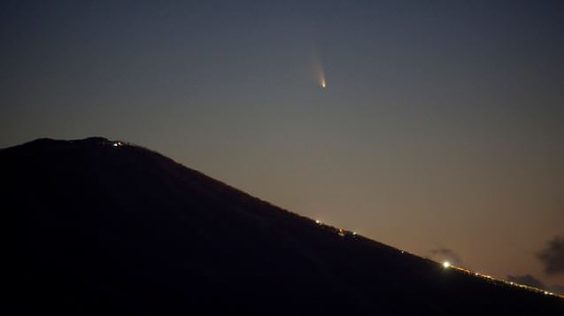
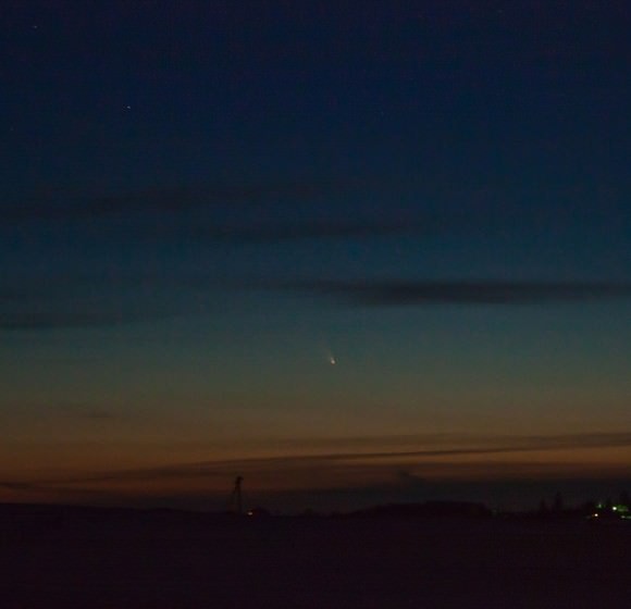
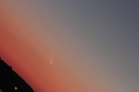
C/2011 L4 (PANSTARRS on March 15, 2013. Taken in Hachimantai City Japan. Credit and copyright: Jason Hill.
You want images and videos of Comet C/2011 L4 (PANSTARRS)? We’ve got ’em! We’ll start with this stunning view from Japan, taken by Jason Hill. But there’s lots more below:
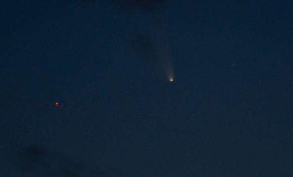
A first capture of Comet PANSTARRS on March 14, 2013. Credit and copyright: Adam Wipp.Another first view of Comet PANSTARRS from Valencia, Spain on March 14, 2013. Credit and copyright: Alejandro Garcia.
This timelapse comes from Andrew Takano, a graduate student at the University of Texas at Austin:
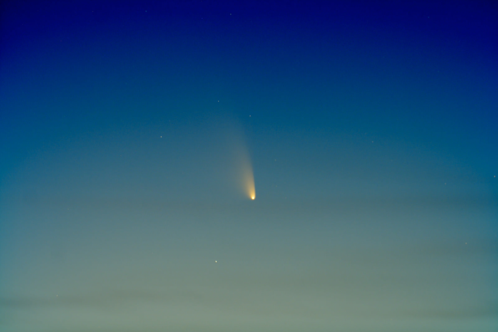
Comet PANSTARRS on March 14, 2013, as seen in the Arizona skies. Credit and copyright: Chris Schur.
Photographer Chris Schur said last night’s views were “the best and brightest comet yet in the western Arizona Sunset sky!” Schur said via email. “I was able to go much deeper tonight using an 80mm Zeiss refractor and Canon Xti. The head shows more fan like protrusions, and the tail is now really shaping up. … The comet here at our elevation of 5150 feet was very easy to see the entire time it was up, and I would rate it at first magnitude for sure.”
Comet PANSTARRS as seen from Aarhus, Denmark (56.2 N, 10.2 E). Credit and copyright: Jens Riggelsen.
Comet Panstarrs above Boulder, Colorado on the evening of March 13, 2013, courtesy of Patrick Cullis:
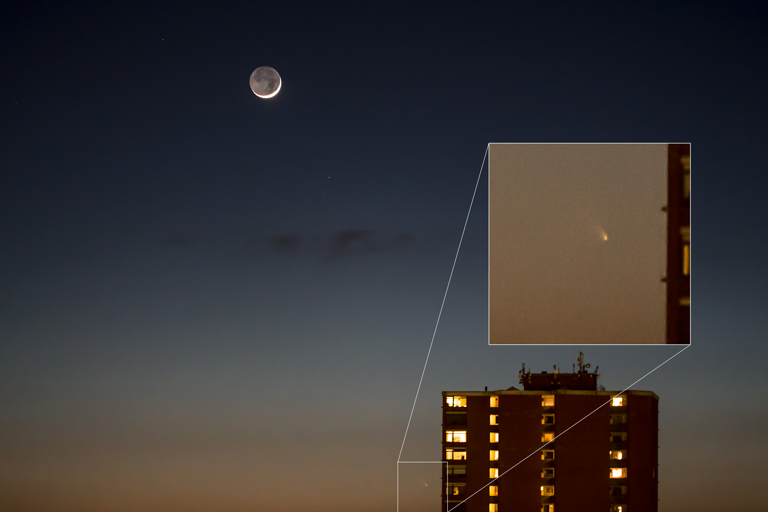
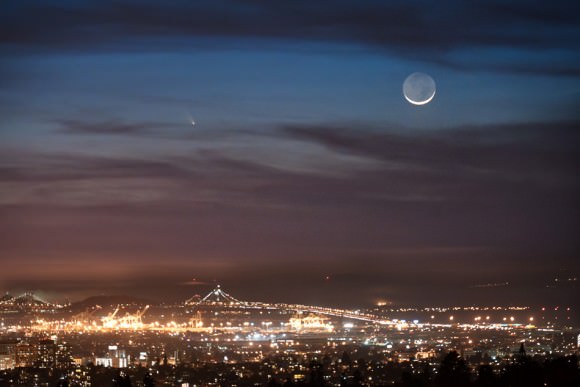
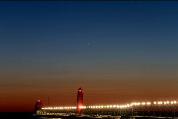
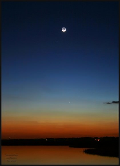
Comet PANSTARRS on March 13, 2013 as see from Newington, New Hampshire, USA. Credit and copyright: John Gianforte (theskyguy.org)Comet PANSTARRS seen from Oakland, California. The Port of Oakland and the Bay Bridge are in the foreground with the comet and crescent moon in the background. Taken on March 12, 2013. Credit and copyright: Jared Wilson.Comet C/2011 L4 (PANSTARRS) floats in the twilight sky over the lighthouses and pier at Grand Haven State Park in Grand Haven, Michigan on March 13, 2013. Credit and copyright: Kevin’s Stuff on Flickr.Comet PANSTARRS and a 5% illuminated Moon on March 13, 2013. Credit and copyright: Tavi Greiner.
You can see more at our Flickr page, and we’ll keep adding and posting! Thanks to everyone who has been so generous with sharing their great photos and videos.
Want to get your astrophoto featured on Universe Today? Join our Flickr group or send us your images by email (this means you’re giving us permission to post them). Please explain what’s in the picture, when you took it, the equipment you used, etc.
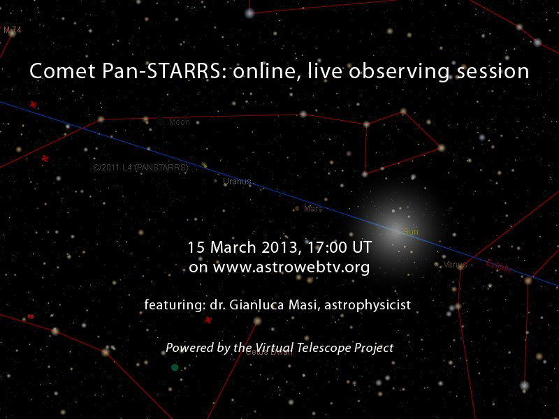
UPDATE: The webcast has been moved to March 16 at 17:00 UTC (1 pm EDT) due to bad weather in Italy.
Has it been cloudy where you live and you haven’t yet been able to see Comet PANSTARRS? The Virtual Telescope Project will have a live webcast of this comet, C/2011 L4 PANSTARRS, from Italy, March 15, on March 16 at 17:00 UTC, 1 p.m. EDT. “We have been waiting for it for over one year, and now the waiting is over,” said astrophysicist Gianluca Masi, who will host the webcast, which you can see at this link. Masi said they are keeping an eye on the skies, and will keep us updated on if they need to change the time of the webcast.
If you’re waiting for the weekend to see it with your own eyes, check out our detailed guides on how to see it here and here. Both are filled with graphics and great info on how to see this comet.
This comet has been a challenge to see, and was actually closest to the Sun on March 10, meaning that is when it was at its brightest. However, while Comet PANSTARRS will fade over the next few weeks, it will also rise higher into a darker sky and become – for a time – easier to see. So keep looking!
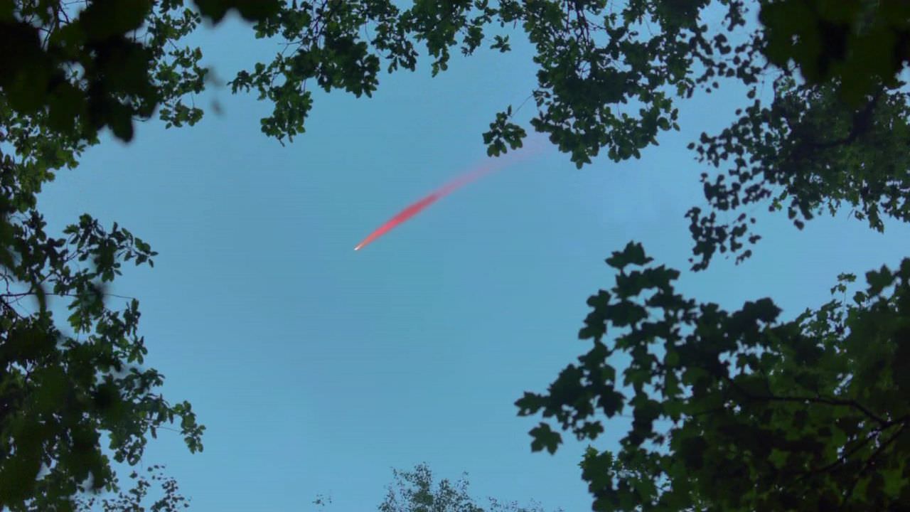
That red comet is pretty, but perhaps not so realistic. Credit: Game of Thrones Wiki/HBO (Screencap)
A blood-red comet appears in the sky. People quake in its wake.
This phenomenon, which happens in the second season of the medieval fantasy Game of Thrones, had us all wondering — can you ever actually see a red comet?
We talked to Matthew Knight, an astronomer at the Lowell Observatory in Arizona who observes comets. He gave us some answers just in time for the third season of Game of Thrones, which begins March 31.
At first blush, he said, the comet’s red color wouldn’t be possible because the strongest emissions from comets are in the blue and green regions, mostly from neutral gases such as hydroxide and cyanide.
There is a type of emission that is close to red, called “forbidden oxygen”, which occurs when atoms make a rare energy transition between states of “excitement”. But it’s very faint and short-lived, Knight wrote.
The visible light from a comet comes from a combination of reflected solar continuum (sunlight reflecting off of dust grains) and cometary emission (neutral and/or ionized molecules of gas that emit photons at a particular wavelength). The sunlight reflecting off of dust grains basically looks like sunlight and since the Sun appears yellow/white, this component cannot look red.
A small caveat is that due to the physical properties of dust grains, comet dust often actually does “redden” sunlight slightly when measured with sensitive equipment. However, this reddening is at a very low level and is not enough to cause the reflected sunlight to appear a deep red like in Game of Thrones. The strongest comet emissions in the region where human eyes can see are in the blue and green regions.
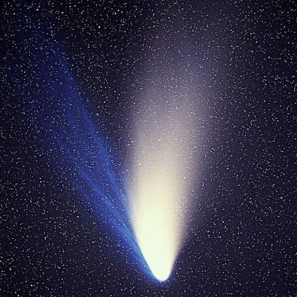
Comet Hale-Bopp. which displays the usual cometary colors. Credit: E. Kolmhofer, H. Raab; Johannes-Kepler-Observatory, Linz, Austria
So what ingredients does a comet need to look like the one in Game of Thrones? According to Knight, it would have to meet these criteria:
Be visible in daylight, which really only happens about once a century;
Be close to the sun (he supposes this one is, given how straight the tail is);
Have a “strange composition” that is different from anything we know in the solar system. The composition could be that forbidden oxygen he talked about, coming from a comet whose ices are carbon monoxide and carbon dioxide. But that would be hard, because those types of ices would not survive long when exposed to sunlight.
If we really want to think in a science fiction vein, Knight suggests that maybe the comet could be made up unpredictably:
Alternatively it could be something else entirely unknown in cometary chemistry or dust, with really weird properties causing a much stronger reddening than is normally seen. In any event, the composition would be so anomalous that this comet would almost certainly have originated in another solar system. That would make comet scientists very interested in studying it!
But don’t despair yet. Comet ISON might be bright enough for daylight viewing when it swings by Earth late in 2013. Comets are unpredictable beasts, but we’re pretty sure of one thing: no matter how bright it is, it won’t look red.
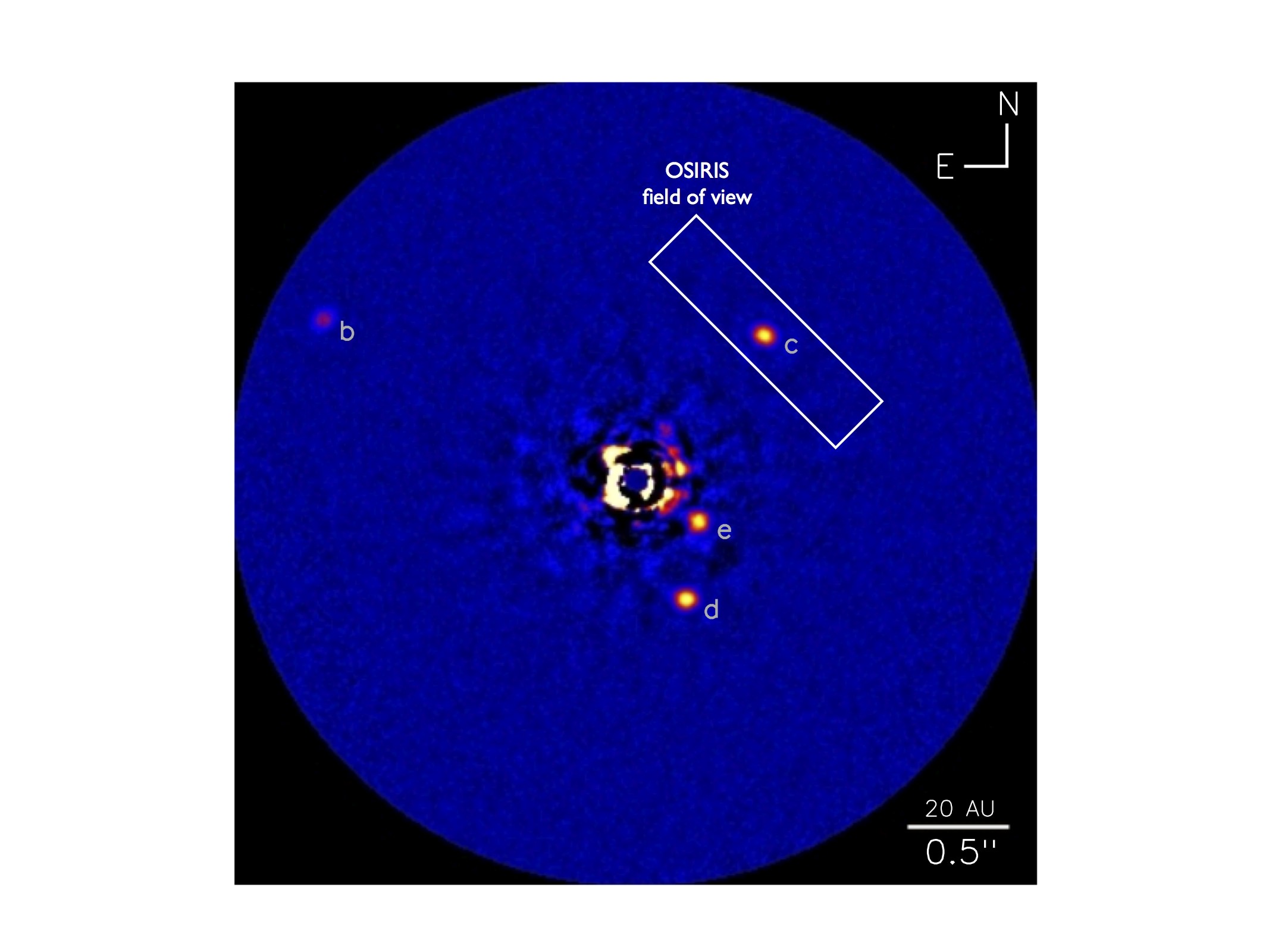
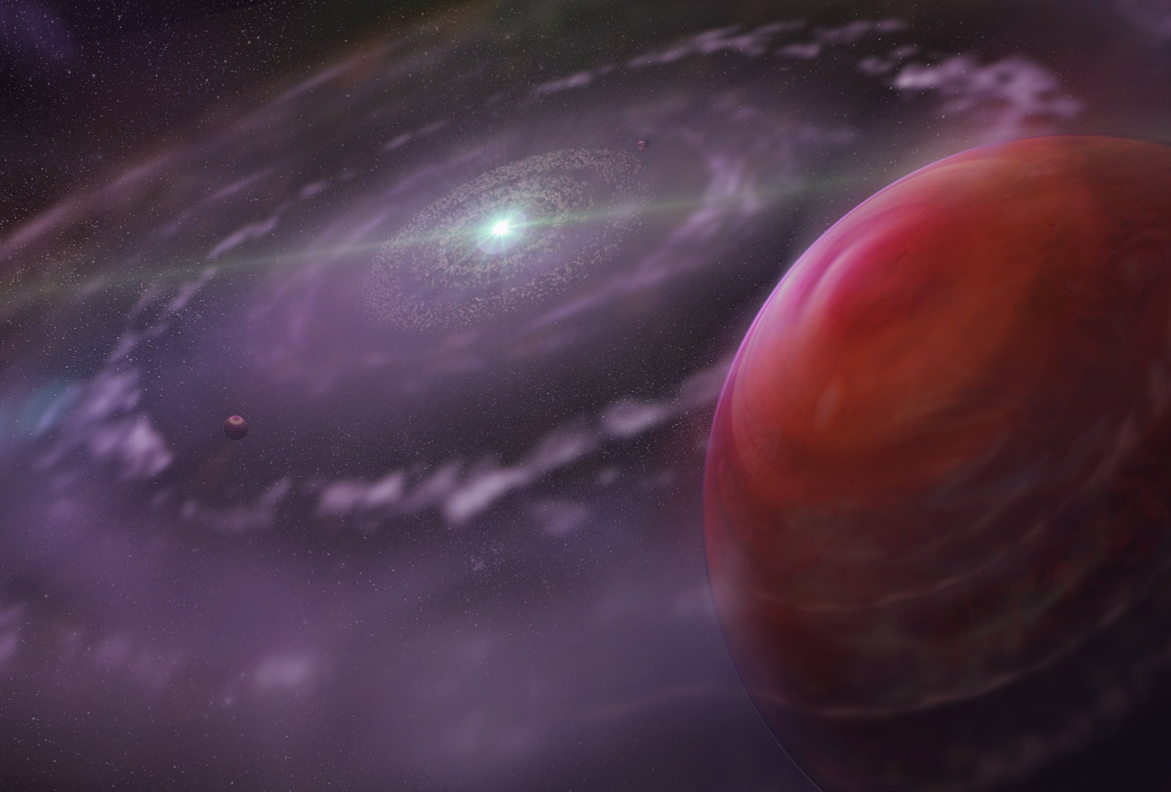
One of the discovery images of the system obtained at the Keck II telescope using the adaptive optics system and NIRC2 Near-Infrared Imager. The rectangle indicates the field-of-view of the OSIRIS instrument for planet C. Credit: Image courtesy of NRC-HIA, C. Marois and Keck Observatory.
The most detailed look yet at the atmosphere of a distant exoplanet has revealed a mixture of water vapor and carbon monoxide blanketing a world ten times the size of Jupiter about 130 light years away from Earth. But even with water present on this world, it is incredibly hostile to life. Like Jupiter, it has no solid surface, and it has a temperature of more than a thousand degree. Additionally, no tell-tale methane signals were detected in the atmosphere. But this solar system is still of great interest, as three other giant worlds orbit the same star and scientists said studying this system will not only help solve mysteries of how it was formed, but also how our own solar system formed as well.
The observations were made at the Keck II telescope in Hawaii, using an infrared imaging spectrograph called OSIRIS, which was able to uncover the chemical fingerprints of specific molecules.
“This is the sharpest spectrum ever obtained of an extrasolar planet,” said Dr. Bruce Macintosh, from the Lawrence Livermore National Laboratory. “This shows the power of directly imaging a planetary system. It is the exquisite resolution afforded by these new observations that has allowed us to really begin to probe planet formation.”
“With this level of detail,” said co-author Travis Barman from the Lowell Observatory, “we can compare the amount of carbon to the amount of oxygen present in the atmosphere, and this chemical mix provides clues as to how the planetary system formed.”
Artist’s rendering of HR 8799c at an early stage in the evolution of the planetary system, showing the planet, a disk of gas and dust, rocky inner planets, and HR 8799. Credit: Dunlap Institute for Astronomy & Astrophysics
The planets around the star, known as HR 8799, weigh in between five to 10 times the mass of Jupiter and are still glowing in infrared with the heat of their formation. The research team says their observations suggest the solar system was created in a similar way to our own, with gas giants forming far away from their parent star and smaller, rocky planets closer in. However, no Earth-like rocky planets have yet been detected in this system.
“The results suggest the HR 8799 system is like a scaled-up Solar System,” said Quinn Kanopacky, an astronomer from the University of Toronto in Canada. “Once the solid cores grew large enough, their gravity quickly attracted surrounding gas to become the massive planets we see today. Since that gas had lost some of its oxygen, the planet ends up with less oxygen and less water than if it had formed through a gravitational instability.”
There are two leading models of planetary formation: core accretion and gravitational instability. When stars form, a planet-forming disk surrounds them. With core accretion, planets form gradually as solid cores slowly grow big enough to start acquiring gas from the disk, while in the gravitational instability model, planets form almost instantly as the disk collapses on itself.
Properties such as the composition of a planet’s atmosphere are clues to how the planet formed, and in this case core accretion seems to win out. Although there was evidence of water vapor, that signature is weaker than would be expected if the planet shared the composition of its parent star. Instead, the planet has a high ratio of carbon to oxygen – a fingerprint of its formation in the gaseous disk tens of millions of years ago. As the gas cooled with time, grains of water ice formed, depleting the remaining gas of oxygen. Planetary formation then began when ice and solids collected into planetary cores.
“Once the solid cores grew large enough, their gravity quickly attracted surrounding gas to become the massive planets we see today,” said Konopacky. “Since that gas had lost some of its oxygen, the planet ends up with less oxygen and less water than if it had formed through a gravitational instability.”
“Spectral information of this quality not only provides clues about the formation of the HR8799 planets but also provides the guidance we need to improve our theoretical understanding of exoplanet atmospheres and their early evolution,” said Barman. “The timing of this work could not be better as it comes on the heels of new instruments that will image dozens more exoplanets, orbiting other stars, that we can study in similar detail.”
This system was also the study as part of remote reconnaissance imaging with Project 1640. The video below explains more:
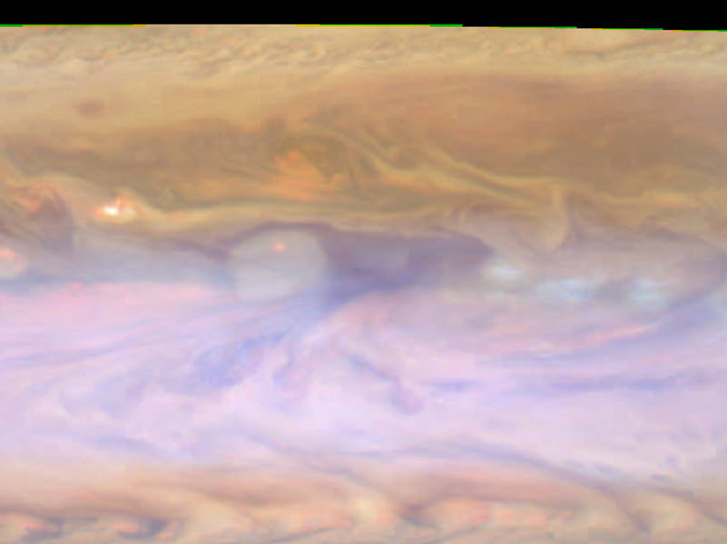
The dark hot spot in this false-color image from NASA's Cassini spacecraft is a window deep into Jupiter's atmosphere. All around it are layers of higher clouds, with colors indicating which layer of the atmosphere the clouds are in. Image credit: NASA/JPL-Caltech/SSI/GSFC
In the swirling canopy of Jupiter’s atmosphere, cloudless patches are so exceptional that the big ones get the special name “hot spots.” Exactly how these clearings form and why they’re only found near the planet’s equator have long been mysteries. Now, using images from NASA’s Cassini spacecraft, scientists have found new evidence that hot spots in Jupiter’s atmosphere are created by a Rossby wave, a pattern also seen in Earth’s atmosphere and oceans. The team found the wave responsible for the hot spots glides up and down through layers of the atmosphere like a carousel horse on a merry-go-round.
“This is the first time anybody has closely tracked the shape of multiple hot spots over a period of time, which is the best way to appreciate the dynamic nature of these features,” said the study’s lead author, David Choi, a NASA Postdoctoral Fellow working at NASA’s Goddard Space Flight Center in Greenbelt, Md. The paper is published online in the April issue of the journal Icarus.
Choi and his colleagues made time-lapse movies from hundreds of observations taken by Cassini during its flyby of Jupiter in late 2000, when the spacecraft made its closest approach to the planet. The movies zoom in on a line of hot spots between one of Jupiter’s dark belts and bright white zones, roughly 7 degrees north of the equator. Covering about two months (in Earth time), the study examines the daily and weekly changes in the sizes and shapes of the hot spots, each of which covers more area than North America, on average.
Much of what scientists know about hot spots came from NASA’s Galileo mission, which released an atmospheric probe that descended into a hot spot in 1995. This was the first, and so far only, in-situ investigation of Jupiter’s atmosphere.
“Galileo’s probe data and a handful of orbiter images hinted at the complex winds swirling around and through these hot spots, and raised questions about whether they fundamentally were waves, cyclones or something in between,” said Ashwin Vasavada, a paper co-author who is based at NASA’s Jet Propulsion Laboratory in Pasadena, Calif., and who was a member of the Cassini imaging team during the Jupiter flyby. “Cassini’s fantastic movies now show the entire life cycle and evolution of hot spots in great detail.”
Because hot spots are breaks in the clouds, they provide windows into a normally unseen layer of Jupiter’s atmosphere, possibly all the way down to the level where water clouds can form. In pictures, hot spots appear shadowy, but because the deeper layers are warmer, hot spots are very bright at the infrared wavelengths where heat is sensed; in fact, this is how they got their name.
One hypothesis is that hot spots occur when big drafts of air sink in the atmosphere and get heated or dried out in the process. But the surprising regularity of hot spots has led some researchers to suspect there is an atmospheric wave involved. Typically, eight to 10 hot spots line up, roughly evenly spaced, with dense white plumes of cloud in between. This pattern could be explained by a wave that pushes cold air down, breaking up any clouds, and then carries warm air up, causing the heavy cloud cover seen in the plumes. Computer modeling has strengthened this line of reasoning.
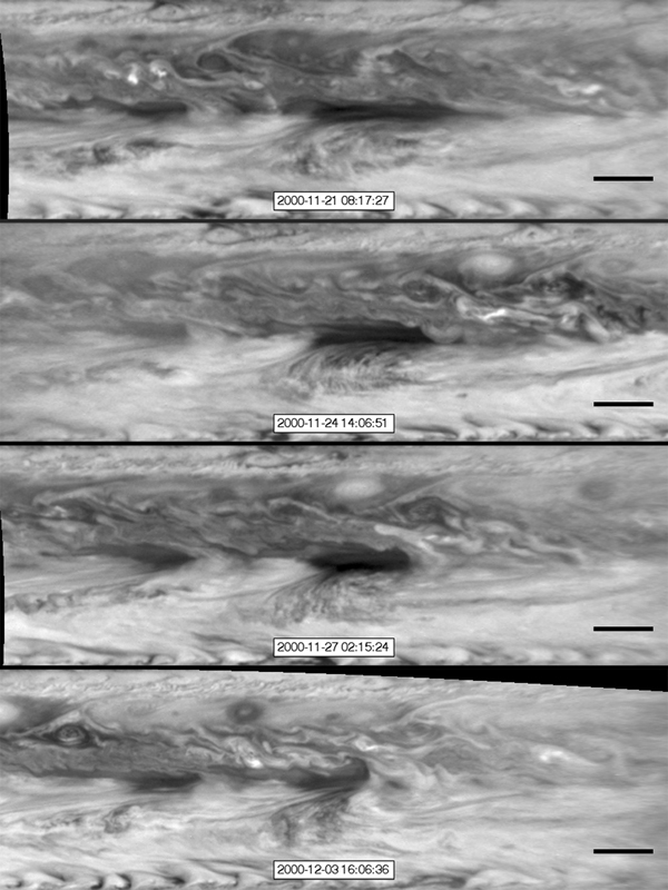
In this series of images from NASA’s Cassini spacecraft, a dark, rectangular hot spot (top) interacts with a line of vortices that approaches from on the upper-right side (second panel). Image credit: NASA/JPL-Caltech/SSI/GSFC
From the Cassini movies, the researchers mapped the winds in and around each hot spot and plume, and examined interactions with vortices that pass by, in addition to wind gyres, or spiraling vortices, that merge with the hot spots. To separate these motions from the jet stream in which the hot spots reside, the scientists also tracked the movements of small “scooter” clouds, similar to cirrus clouds on Earth. This provided what may be the first direct measurement of the true wind speed of the jet stream, which was clocked at about 300 to 450 mph (500 to 720 kilometers per hour) — much faster than anyone previously thought. The hot spots amble at the more leisurely pace of about 225 mph (362 kilometers per hour).
By teasing out these individual movements, the researchers saw that the motions of the hot spots fit the pattern of a Rossby wave in the atmosphere. On Earth, Rossby waves play a major role in weather. For example, when a blast of frigid Arctic air suddenly dips down and freezes Florida’s crops, a Rossby wave is interacting with the polar jet stream and sending it off its typical course. The wave travels around our planet but periodically wanders north and south as it goes.
The wave responsible for the hot spots also circles the planet west to east, but instead of wandering north and south, it glides up and down in the atmosphere. The researchers estimate this wave may rise and fall 15 to 30 miles (24 to 50 kilometers) in altitude.
The new findings should help researchers understand how well the observations returned by the Galileo probe extend to the rest of Jupiter’s atmosphere. “And that is another step in answering more of the questions that still surround hot spots on Jupiter,” said Choi.
If you’re reading this then you probably love space exploration, and if you love space exploration then you know how awesome the MESSENGER mission is — the incredibly successful venture by NASA, Johns Hopkins University Applied Physics Laboratory, and the Carnegie Institution of Washington to orbit and study the first rock from the Sun in unprecedented detail. Since entering orbit around Mercury on March 18, 2011, MESSENGER has mapped nearly 100% of the planet’s surface, found unique landforms called hollows residing in many of its craters, and even discovered evidence of water ice at its poles! That’s a lot to get accomplished in just two years!
The video above, assembled by Mark ‘Indy’ Kochte, is a tribute to the many impressive achievements of the MESSENGER mission, featuring orbital animations (love that MESSENGER shimmy!), surface photos, and the approach to the planet. Enjoy!
Images and animation stills courtesy NASA/Johns Hopkins University Applied Physics Laboratory/Carnegie Institution of Washington. Music: “Mercury Ridge” by Simon Wilkinson. Video creation and time-lapse animations by Mark ‘Indy’ Kochte.