The Milky Way’s Magnetic Personality

The sky map of the Faraday effect caused by the magnetic fields of the Milky Way. Red and blue colors indicate regions of the sky where the magnetic field points toward and away from the observer, respectively. The band of the Milky Way (the plane of the Galactic disk) extends horizontally in this panoramic view. The center of the Milky Way lies in the middle of the image. The North celestial pole is at the top left and the South Pole is at the bottom right. (Image Credit: Max Planck Institute for Astrophysics)

[/caption]

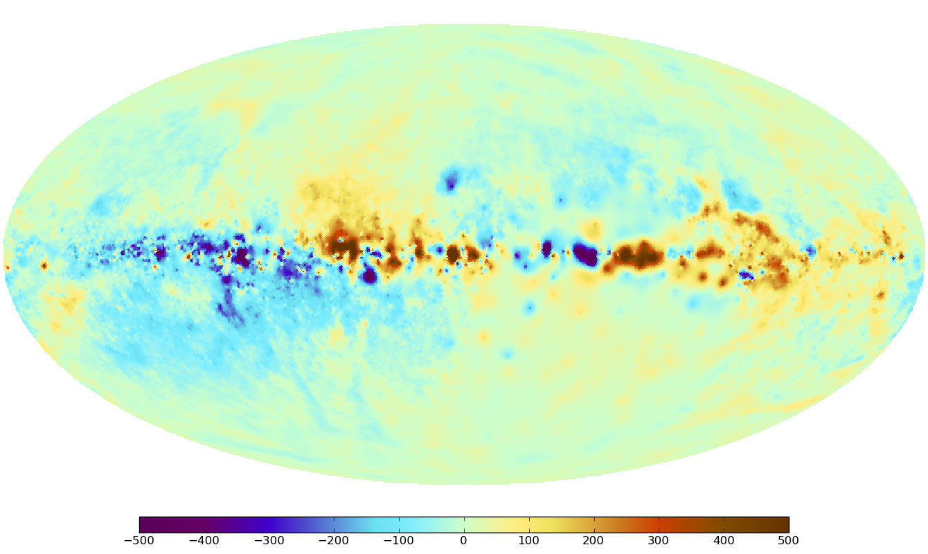
Recently we took a look at a very unusual type of map – the Faraday Sky. Now an international team of scientists, including those at the Naval Research Laboratory, have pooled their information and created one of the most high precision maps to date of the Milky Way’s magnetic fields. Like all galaxies, ours has a magnetic “personality”, but just where these fields come from and how they are created is a genuine mystery. Researchers have always simply assumed they were created by mechanical processes like those which occur in Earth’s interior and the Sun. Now a new study will give scientists an even better understanding about the structure of galactic magnetic fields as seen throughout our galaxy.

The team, led by the Max Planck Institute for Astrophysics (MPA), gathered their information and compiled it with theoretical simulations to create yet another detailed map of the magnetic sky. As NRL’s Dr. Tracy Clarke, a member of the research team explains, “The key to applying these new techniques is that this project brings together over 30 researchers with 26 different projects and more than 41,000 measurements across the sky. The resulting database is equivalent to peppering the entire sky with sources separated by an angular distance of two full moons.” This huge amount of data provides a new “all-sky” look which will enable scientists to measure the magnetic structure of the Milky Way in minute detail.

In this map of the sky, a correction for the effect of the Galactic disk has been made in order to emphasize weaker magnetic field structures. The magnetic field directions above and below the disk seem to be diametrically opposed, as indicated by the positive (red) and negative (blue) values. An analogous change of direction takes place across the vertical center line, which runs through the center of the Milky Way. (Image Credit: Max Planck Institute for Astrophysics)
Just what’s so “new” about this map? This time we’re looking at a quantity called Faraday depth – an idea dependent on a line-of-sight information set on the magnetic fields. It was created by combining more than 41,000 singular measurements which were then combined using a new image reconstruction method. In this case, all the researchers at MPA are specialists in the new discipline of information field theory. Dr. Tracy Clarke, working in NRL’s Remote Sensing Division, is part of the team of international radio astronomers who provided the radio observations for the database. It’s magnetism on a grand scale… and imparts even the smallest of magnetic features which will enable scientists to further understand the nature of galactic gas turbulence.

The concept of the Faraday effect isn’t new. Scientists have been observing and measuring these fields for the last century and a half. Just how is it done? When polarized light passes through a magnetized medium, the plane of the polarization flips… a process known as Faraday rotation. The amount of rotation shows the direction and strength of the field and thereby its properties. Polarized light is also generated from radio sources. By using different frequencies, the Faraday rotation can also be measured in this alternative way. By combining all of these unique measurements, researchers can acquire information about a single path through the Milky Way. To further enhance the “big picture”, information must be gathered from a variety of sources – a need filled by 26 different observing projects that netted a total of 41,330 individual measurements. To give you a clue of the size, that ends up being about one radio source per square degree of sky!

The uncertainty in the Faraday map. Note that the range of values is significantly smaller than in the Faraday map (Fig. 1). In the area of the celestial south pole, the measurement uncertainties are particularly high because of the low density of data points. (Image Credit: Max Planck Institute for Astrophysics)
Even with depth like this, there are still areas in the southern sky where only a few measurements have been cataloged. To fill in the gaps and give a more realistic view, researchers “have to interpolate between the existing data points that they have recorded.” However, this type of data causes some problems with accuracy. While you might think the more exact measurements would have the greatest impact on the map, scientists aren’t quite sure how reliable any single measurement could be – especially when they could be influenced by the environment around them. In this case, the most accurate measurements don’t always rank the highest in mapping points. Like Heisenberg, there’s an uncertainty associated with the process of obtaining measurements because the process is so complex. Just one small mistake could lead to a huge distortion in the map’s contents.

Thanks to an algorithm crafted by the MPA, scientists are able to face these types of difficulties with confidence as they put together the images. The algorithm, called the “extended critical filter,” employs tools from new disciplines known as information field theory – a logical and statistical method applied to fields. So far it has proven to be an effective method of weeding out errors and has even proven itself to be an asset to other scientific fields such as medicine or geography for a range of image and signal-processing applications.

Even though this new map is a great assistant for studying our own galaxy, it will help pave the way for researchers studying extragalactic magnetic fields as well. As the future provides new types of radio telescopes such as LOFAR, eVLA, ASKAP, MeerKAT and the SKA , the map will be a major resource of measurements of the Faraday effect – allowing scientists to update the image and further our understanding of the origin of galactic magnetic fields.

Original Story Source: Naval Research Laboratory News.

Journal Club – Neutrino Vision

Today's Journal Club is about a new addition to the Standard Model of fundamental particles.

[/caption]

According to Wikipedia, a journal club is a group of individuals who meet regularly to critically evaluate recent articles in the scientific literature. And of course, the first rule of Journal Club is… don’t talk about Journal Club.

So, without further ado – today’s journal article is about the latest findings in neutrino astronomy.

Today’s article:
Gaisser Astrophysical neutrino results..

This paper presents some recent observations from the IceCube neutrino telescope at the South Pole – which acually observes neutrinos from the northern sky – using the Earth to filter out some of the background noise. Cool huh?

Firstly, a quick recap of neutrino physics. Neutrinos are sub-atomic particles of the lepton variety and are essentially neutrally charged versions of the other leptons – electrons, muons and taus – which all have a negative charge. So, we say that neutrinos come in three flavours – electron neutrinos, muon neutrinos and tau neutrinos.

Neutrinos were initially proposed by Pauli (a proposal later refined by Fermi) to explain how energy could be transported away from a system undergoing beta decay. When solar fusion began to be understood in the 1930s – the role of neutrinos was problematic since only a third or more of the neutrinos that were predicted to be produced by fusion were being detected – an issue which became known as the solar neutrino problem in the 1960’s.

The solar neutrino problem was only resolved in the late 1990s when the three neutrino flavours idea gained wide acceptance and each were finally detected in 2001 – confirming that solar neutrinos in transit actually oscillate between the three flavours (electron, muon and tau) – which means that if your detector is set up to detect only one flavour you will detect only about one third of all the neutrinos coming from the Sun.

Ten years later, the Ice Cube the neutrino observatory is using our improved understanding of neutrinos to try and detect high energy neutrinos of extragalactic origin. The first challenge is to distinguish atmospheric neutrinos (produced in abundance as cosmic rays strike the atmosphere) from astrophysical neutrinos.

Using what we have learnt from solving the solar neutrino problem, we can be confident that any neutrinos from distant sources have had time to oscillate – and hence should arrive at Earth in approximately equal ratios. Atmospheric neutrinos produced from close sources (also known as ‘prompt’ neutrinos) don’t have time to oscillate before being detected.

When looking for point sources of high energy astrophysical neutrinos, IceCube is most sensitive to muon neutrinos – which are detected when the neutrino weakly interacts with an ice molecule – emitting a muon. A high energy muon will then generate Cherenkov radiation – which is what IceCube actually detects. Unfortunately muon neutrinos are also the most common source of cosmic ray induced atmospheric neutrinos, but we are steadily getting better at determining what energy levels represent astrophysical rather than atmospheric neutrinos.

So, it’s still early days with this technology – with much of the effort going in to learning how to observe, rather than just observing. But maybe one day we will be observing the cosmic neutrino background – and hence the first second of the Big Bang. One day…

So… comments? Are neutrinos the fundamentally weirdest fundamental particle out there? Could IceCube be used to test the faster-than-light neutrino hypothesis? Want to suggest an article for the next edition of Journal Club?

Recycling Pulsars – The Millisecond Matters…

An artist's impression of an accreting X-ray millisecond pulsar. The flowing material from the companion star forms a disk around the neutron star which is truncated at the edge of the pulsar magnetosphere. Credit: NASA / Goddard Space Flight Center / Dana Berry

[/caption]

It’s a millisecond pulsar… a rapidly rotating neutron star and it’s about to reach the end of its mass gathering phase. For ages the vampire of this binary system has been sucking matter from a donor star. It has been busy, spinning at incredibly high rotational speeds of about 1 to 10 milliseconds and shooting off X-rays. Now, something is about to happen. It is going to lose a whole lot of energy and age very quickly.

Astrophysicist Thomas Tauris of Argelander-Institut für Astronomie and Max-Planck-Institut für Radioastronomie has published a paper in the February 3 issue of Science where he has shown through numerical equations the root of stellar evolution and accretion torques. In this model, millisecond pulsars are shown to dissipate approximately half of their rotational energy during the last phase of the mass-transfer process and just before it turns into a radio source. Dr. Tauris’ findings are consistent with current observations and his conclusions also explain why a radio millisecond pulsar appears age-advanced over their companion stars. This may be the answer as to why sub-millisecond pulsars don’t exist at all!

“Millisecond pulsars are old neutron stars that have been spun up to high rotational frequencies via accretion of mass from a binary companion star.” says Dr. Tauris. “An important issue for understanding the physics of the early spin evolution of millisecond pulsars is the impact of the expanding magnetosphere during the terminal stages of the mass-transfer process.”

By drawing mass and angular momentum from a host star in a binary system, a millisecond pulsar lives its life as a highly magnetized, old neutron star with an extreme rotational frequency. While we might assume they are common, there are only about 200 of these pulsar types known to exist in galactic disk and globular clusters. The first of these millisecond pulsars was discovered in 1982. What counts are those that have spin rates between 1.4 to 10 milliseconds, but the mystery lay in why they have such rapid spin rates, their strong magnetic fields and their strangely appearing ages. For example, when do they switch off? What happens to the spin rate when the donor star quits donating?

“We have now, for the first time, combined detailed numerical stellar evolution models with calculations of the braking torque acting on the spinning pulsar”, says Thomas Tauris, the author of the present study. “The result is that the millisecond pulsars lose about half of their rotational energy in the so-called Roche-lobe decoupling phase. This phase is describing the termination of the mass transfer in the binary system. Hence, radio-emitting millisecond pulsars should spin slightly slower than their progenitors, X-ray emitting millisecond pulsars which are still accreting material from their donor star. This is exactly what the observational data seem to suggest. Furthermore, these new findings can help explain why some millisecond pulsars appear to have characteristic ages exceeding the age of the Universe and perhaps why no sub-millisecond radio pulsars exist.”

Thanks to this new study we’re now able to see how a spinning pulsar could possibly brake out of an equilibrium spin. At this age, the mass-transfer rate slows down and affects the magnetospheric radius of the pulsar. This in turn expands and forces the incoming matter to act as a propeller. The action then causes the pulsar to slow down its rotation and – in turn – slow its spin rate.

“Actually, without a solution to the “turn-off” problem we would expect the pulsars to even slow down to spin periods of 50-100 milliseconds during the Roche-lobe decoupling phase”, concludes Thomas Tauris. “That would be in clear contradiction with observational evidence for the existence of millisecond pulsars.”

Original Story Source: Max-Planck-Institut für Radioastronomie News Release>. For Further Reading: Spin-Down of Radio Millisecond Pulsars at Genesis.

New Study Shows How Trace Elements Affect Stars’ Habitable Zones

Comparison of the habitable zone around the Sun in our solar system and around the star Gliese 581. Credit: ESO

[/caption]

Habitable zones are the regions around stars, including our own Sun, where conditions are the most favourable for the development of life on any rocky planets that happen to orbit within them. Generally, they are regions where temperatures allow for liquid water to exist on the surface of these planets and are ideal for “life as we know it.” Specific conditions, due to the kind of atmosphere, geological conditions, etc. must also be taken into consideration, on a case-by-case basis.

Now, by examining trace elements in the host stars, researchers have found clues as to how the habitable zones evolve, and how those elements also influence them. To determine what elements are in a star, scientists study the wavelengths of its light. These trace elements are heavier than the hydrogen and helium gases which the star is primarily composed of. Variations in the composition of these stars are now thought to affect the habitable zones around them.

The study was led by Patrick Young, a theoretical astrophysicist and astrobiologist at Arizona State University. Young and his team presented their findings on January 11, 2012 at the annual meeting of the American Astronomical Society in Austin, Texas. He and his colleagues have examined more than a hundred dwarf stars so far.

An abundance of these elements can affect how opaque a star’s plasma is. Calcium, sodium, magnesium, aluminum and silicon have been found to also have small but significant effects on a star’s evolution – higher levels tended to result in cooler, redder stars. As Young explains, “The persistence of stars as stable objects relies on the heating of plasma in the star by nuclear fusion to produce pressure that counteracts the inward force of gravity. A higher opacity traps the energy of fusion more efficiently and results in a larger radius, cooler star. More efficient use of energy also means that nuclear burning can proceed more slowly, resulting in a longer lifetime for the star.”

The lifetime of a star’s habitable zone can also be influenced by another element – oxygen. Young continues: “The habitable lifetime of an orbit the size of Earth’s around a one-solar-mass star is only 3.5 billion years for oxygen-depleted compositions but 8.5 billion years for oxygen-rich stars. For comparison, we expect the Earth to remain habitable for another billion years or so, for about 5.5 billion years total, before the Sun becomes too luminous. Complex life on Earth arose some 3.9 billion years after its formation, so if Earth is at all representative, low-oxygen stars are perhaps less than ideal targets.”

As well as the habitable zone, the composition of a star can determine the eventual composition of any planets that form. The carbon-oxygen and magnesium-silicon ratios of stars can affect whether a planet will have magnesium or silicon-loaded clay minerals such as magnesium silicate (MgSiO3), silicon dioxide (SiO2), magnesium orthosilicate (Mg2SiO4), and magnesium oxide (MgO). A star’s composition can also play a role in whether a rocky planet might have carbon-based rock instead of silicon-based rock like our planet. Even the interior of planets could be affected, as radiocative elements would determine whether a planet has a molten core or a solid one. Plate tectonics, thought to be important for the evolution of life on Earth, depend on a molten interior.

Young and his team are now looking at 600 stars, ones that are already being targeted in exoplanet searches. They plan to produce a list of the 100 best stars which could have potentially habitable planets.

Beautiful Conjunction: Comet Garradd Meets M92

This lovely image of Comet Garradd (C/2009 PI) as it passes by the globular cluster M92 in the constellation Hercules, was taken remotely from the Tzek Maun Observatory in New Mexico by our friends Giovanni Sostero, Ernest Guido and Nick Howes. While the two objects look like they are right next to each other, M92 is over 25,000 light-years away while Comet Garradd is 12.5 light-minutes away from Earth! The comet looks almost like a bird or winged starship in flight with the dust tail and ion tail shooting off on either side. Comet Garradd is still on show in the northern hemisphere, although you’ll at least need binoculars to see it. The comet is around magnitude 7 now, and is heading north, so over the course of the next few weeks, it should become a little easier to see. For now, you need to get up early to see it, (around 5:30 to 6:30 am), but by the end of the month it should be visible all night long.

You can see another image of Garradd on today’s APOD (but personally I really like the one right here!)

Cities at Night Panorama of Millions of US East Coast Earthlings

Nighttime Panorama of US East Coast from the ISS. Astronauts aboard the International Space Station (ISS) captured this stunning nighttime panorama of the major cities along the East Coast of the United States on Jan. 29. Credit: NASA

[/caption]

Do you live here?

Tens of millions of Earthlings live and work in the bustling and seemingly intertwined American mega-metropolis of the Philadelphia-New York City-Boston corridor (bottom-center splotch) captured in this stunning “Cities at Night” panorama of the East Coast of the United States along the Atlantic seaboard (image above).

Look northward and you’ll see the home to millions more Earthlings inhabiting the brilliantly lit Canadian cities of Toronto (launch site for “Lego Man in Space“) and Montreal to the west of Lake Ontario (dark oval at left-center).

The gorgeous panorama showing a portion of the Earth at Night and the atmospheric limb and light activity from the Aurora Borealis was snapped by the Expedition 30 crew living and working aboard the million pound International Space Station (ISS) on Jan. 29.

Lately, the 6 man international crew of Expedition 30 from Russia, Holland and the US have been on a roll taking one after another magnificent Nighttime pictures of our Home Planet, Auroras’ and celestial wonders like Comet Lovejoy.

Be sure to take a comparative look at the recent panorama of Western Europe at Night snapped by the ISS crew a week before on Jan 22 – here.

To test your geography smarts, here’s a map of the US East Coast highlighting much of what’s visible in the ISS panorama.

This Earthling has lived in cities on the US East Coast and Western Europe – images above and below

Western Europe at Night
European ‘Cities at Night’ from the ISS with station solar arrays and robotic hand in foreground. Credit: NASA

Two years ago in Feb. 2010, the US East Coast was struck by “Snowmageddon”, and this is how we looked from space

Meanwhile, two of the Expedition 30 crew members, Russian Flight Engineers Oleg Kononenko and Anton Shkaplerov, are preparing for a spacewalk on Friday, Feb. 16. They will be installing equipment outside the ISS on the Russian Pirs, Poisk and Zvezda modules.

Incredible 3-D View Inside a Martian Crater

A 3-d view of a well-preserved and unnamed impact crater on Mars, as seen by the HiRISE camera on the Mars Reconnaisancee Orbiter. Credit: NASA/JPL/University of Arizona. Click for high-resolution version.

[/caption]

This is why I always keep a pair of 3-D glasses by my computer. This well-preserved crater on Mars may look like just your average, run-of-the-mill impact crater in 2-D, but in 3-D, the sharply raised rim, the deep, cavernous crater body, and especially the steep crater walls will have you grabbing your armchairs so you don’t fall in. The image is courtesy of the HiRISE camera team from the Mars Reconnaissance Orbiter. This unnamed crater is about 6 or 7 kilometers wide from rim to rim. HiRISE took the image on New Year’s Eve 2011.

HiRISE principal investigator Alfred McEwen says that the camera has imaged hundreds of well-preserved impact craters on Mars ranging from 1 meter to more than 100 kilometers wide. What can the scientists learn from craters?

“These targets are of great interest for multiple reasons,” he said. “First, we want to better understand impact cratering, a fundamental surface process. Second, such craters often contain good exposures of bedrock in the steep walls and, if the crater is large enough, in the central uplift. Just like terrestrial geologists are attracted to good bedrock outcrops like road cuts, planetary geologists are attracted to well-preserved craters.

“Third, the steep slopes often reveal active processes, such as formation of gullies, boulder falls, and slope streaks that could form in a variety of ways. Some of these active processes could be related to water, since the crater may expose lenses of ice or salty water, or create deep shadows that trap volatiles, or expose salts that can extract water from the air.”

Plus, they are just plain wonderful to behold, especially in the resolution the HiRISE can obtain.

A non-3-D version of the same image. Credit: NASA/JPL/University of Arizona

Source: HiRISE

Can We Land On a Comet?

An artist concept of the Philae lander on comet 67P/Churyumov-Gerasimenko. Credit: Astrium - E. Viktor/ESA

The Rosetta mission will do something never before attempted: land on a comet. The spacecraft is now on its way to intercept comet 67P/Churyumov-Gerasimenko in January 2014 and land a probe on it for what promises to be an amazing view. But what we know of comets so far comes from a few flyby missions. So, with surface composition and conditions largely a mystery, so how did engineers prepare to land on something that could be either solid ice or rock, or a powdery snow or regolith – or something in between?

They had to design the Philae lander so it could land equally well on any surface. In the tiny gravitational field of a comet, landing on hard icy surface might cause Philae to bounce off again. Alternatively, hitting a soft snowy one could result in it sinking. To cope with either possibility, Philae will touch as softly as possible. In fact, engineers have likened it more to docking in space.

Philae will fire harpoons to secure itself to the comet; additionally, the landing gear is equipped with large pads to spread its weight across a broad area (kind of like snowshoes.)

While landing on a comet will certainly be nail-biting, having a front row seat for when the comet gets closer to the Sun is the most highly anticipated part of the mission.

[/caption]

“In some ways, a flyby is just a tantalizing glimpse of a comet at one stage in its evolution,” says Claudia Alexander, project scientist for the U.S. Rosetta Project at JPL. “Rosetta is different. It will orbit 67P for 17 months. We’ll see this comet evolve right before our eyes as we accompany it toward the Sun and back out again.”

We’ll be able to watch as it becomes “something poetic and beautiful, trailing a vast tail,” said Alexander. For once, we’ll be able to watch the surface of a comet transform in front of our eyes instead of relying on artist concept drawings! Additionally, the Rosetta spacecraft up above will be busy mapping the comet’s surface and magnetic field, monitoring the comet’s erupting jets and geysers, measuring outflow rates, and much more. Together, the orbiter and lander will build up the first 3-D picture of the layers and pockets under the surface of a comet.

Comets are considered a gold mine for astronomers who want to know what conditions were like back in the early days of our Solar System. And the data and images from this mission promises to be some of the most stunning we’ve yet seen.

Find out more about the Rosetta mission in the accompanying video, or see the ESA Rosetta website.

Source: Science@NASA

Are You Listening to Astronomy.FM?

Are you listening to Astronomy.FM? If not, you should join the audience of over 25,000 listeners in 85 countries who are enjoying this amazing free service. Astronomy.FM is billed as “The only all-Astronomy radio station in the Known Universe.” You can listen to this one-of-a-kind radio station on-line anytime, as it is streaming 24 hours a day and it includes both wonderful original astronomy programming and replays of many great astronomy shows and podcasts including Astronomy Cast, 365 Days of Astronomy, Planetary Radio, 60-Second Science and Slacker Astronomy, and also they have just recently added the Weekly Space Hangouts to their lineup. They also have science and astronomy news – the kind of stuff you really want to hear! (As Astronomy.FM announcer Rob Berthiaume said, “Who cares about Snooki? Give me more supernovae!”

What is really awesome about Astronomy.FM (besides their great programming) is that it is an all-volunteer organization. Everyone who you hear on-air does it for their love of astronomy.

Right now, Astronomy.FM is having their annual funding drive. They are trying to raise $6,000 for their annual budget. Can you imagine – running a 24-hour radio station for just $6,000 USD?? All revenue is spent on hardware, software, radio programming, and broadcast bandwidth. And 100% of their operational costs are funded solely by listener donations. They receive no government or commercial support, and none of their team members are paid. But, as you can imagine, the streaming fees alone are significant. In addition, with their growing listenership, they also are in need of a back-up server and advanced digital broadcast technology.

Astronomy.FM has some wonderful talent. On-air personality and Program Director Michael Foerster has an amazing voice that I could listen to all day, as well as having a wealth of knowledge about space and astronomy. Rob Keown, Tavi Greiner, and Marleen Bryan are also just some of the other wonderful voices you’ll hear on Astronomy.FM.

If you are already a listener, please consider donating to make sure this great service can remain online. If you aren’t familiar with Astronomy.FM, check it out, and enjoy all their great programming. And then consider supporting it. If you are interested in sharing your talents, here’s the “Contact” page for Astronomy.FM

Anything you can contribute will make a big difference, as they need to make their goal of $6,000 soon. I just donated and I hope you will too.

How Plants May Have Helped Create Earth’s Unique Landscapes

Credit: Wikimedia Commons

[/caption]

According to conventional thinking, plant life first took hold on Earth after oceans and rivers formed; the soil produced by liquid water breaking down bare rock provided an ideal medium for plants to grow in. It certainly sounds logical, but a new study is challenging that view – the theory is that vascular plants, those containing a transport system for water and nutrients, actually created a cycle of glaciation and melting, conditions which led to the formation of rivers and mud which allowed forests and farmland to later develop. In short, they helped actually create the landscapes we see today.

The evidence was just published in two articles in a special edition of Nature Geoscience.

In the first article, analysis of the data proposes that vascular plants began to absorb the carbon dioxide in the atmosphere about 450 million years ago. This led to a cooling of temperatures on a global scale, resulting in widespread glaciation. As the glaciers later started to melt, they ground up the Earth’s surface, forming the kind of soils we see today.

The second article goes further, stating that today’s rivers were also created by vascular plants – the vegetation broke the rocks down into mud and minerals and then also held the mud in place. This caused river banks to start forming, acting as channels for water, which up until then had tended to flow over the surface much more randomly. As the water was channeled into more specific routes, rivers formed. This led to periodic flooding; sediments were deposited over large areas which created rich soil. As trees were able to take root in this new soil, debris from the trees fell into the rivers, creating logjams. This had the effect of creating new rivers and causing more flooding. These larger fertile areas were then able to support the growth of larger lush forests and farmland.

According to Martin Gibling, a professor of Earth science at Dalhousie University, “Sedimentary rocks, before plants, contained almost no mud. But after plants developed, the mud content increased dramatically. Muddy landscapes expanded greatly. A new kind of eco-space was created that wasn’t there before.”

The new theory also leads to the possibility that any exoplanets that happen to have vegetation would look different from Earth; varying circumstances would create a surface unique to each world. Any truly Earth-like exoplanets might be very similar in general, but the way that their surfaces have been modified might be rather different.

It’s an interesting scenario, but it also raises other questions. What about the ancient river channels on Mars? Some appear to have been formed by brief catastrophic floods, but others seem more similar to long-lived rivers here on Earth, especially if there actually was a northern hemisphere ocean as well. How did they form? Does this mean that rivers could form in a variety of ways, with or without plant life being involved? Could Mars have once had something equivalent to vascular plant life as well? Or could the new theory just be wrong? Then there’s Titan, which has numerous rivers still flowing today. Albeit they are liquid methane/ethane instead of water, but what exactly led to their formation?

From the editorial in Nature Geoscience:

Without the workings of life, the Earth would not be the planet it is today. Even if there are a number of planets that could support tectonics, running water and the chemical cycles that are essential for life as we know it, it seems unlikely that any of them would look like Earth. Even if evolution follows a predictable path, filling all available niches in a reproducible and consistent way, the niches on any Earth analogue could be different if the composition of its surface and atmosphere are not identical to those of Earth. And if evolution is random, the differences would be expected to be even larger. Either way, a glimpse of the surface of an exoplanet — if we ever get one — may give us a whole new perspective on biogeochemical cycling and geomorphology.

Just as the many exoplanets now being found are of a previously unknown and amazingly wide variety, and all uniquely alien, even the ones that (may) support life are likely to be just as diverse from each other as they are from Earth itself. Earth’s “twin” may be out there, but in terms of outward appearance, it may be somewhat more of a fraternal twin than an exact replica.