As the “V” in the designation of V445 Puppis indicates, this star was a variable star located in the constellation of Puppis. It was a fairly ordinary periodic variable, although with a rather complex light curve, but still showing a distinct periodicity of about fifteen and a half hours. It wasn’t especially bright, yet something seemed to tug at my memory regarding the star’s name as I scanned through articles to write on. Just over a year ago, Nancy wrote a post on V445 Puppis stating it’s a supernova just waiting to happen. A new article challenges this claim.
In December of 2000, V445 Puppis underwent an unusual nova. It was first noticed on December 30th, but archival records showed the eruption began in early November of that year and reached a peak brightness on November 29th. The system was known to be a binary star system with a shared envelope in which the primary star was a white dwarf and thus, a nova was the most readily available explanation.
However, this wasn’t a normal nova. Spectroscopic observations early the next year showed the ejecta lacked the helium emission seen in classical novae in which hydrogen piles up on a white dwarf surface until it undergoes fusion into helium. Instead, astronomers saw lines of iron, calcium, carbon, sodium, and oxygen expanding at nearly 1,000 km/sec. This fit better with a proposed type of explosion where, instead of hydrogen collecting on the dwarf’s surface, it was helium and the eruption seen was a helium flash in which it was helium that underwent fusion. Slowly the star faded, and debris from the eruption cooled to form dust. Today, the star itself is completely obscured in the visible portion of the spectrum.
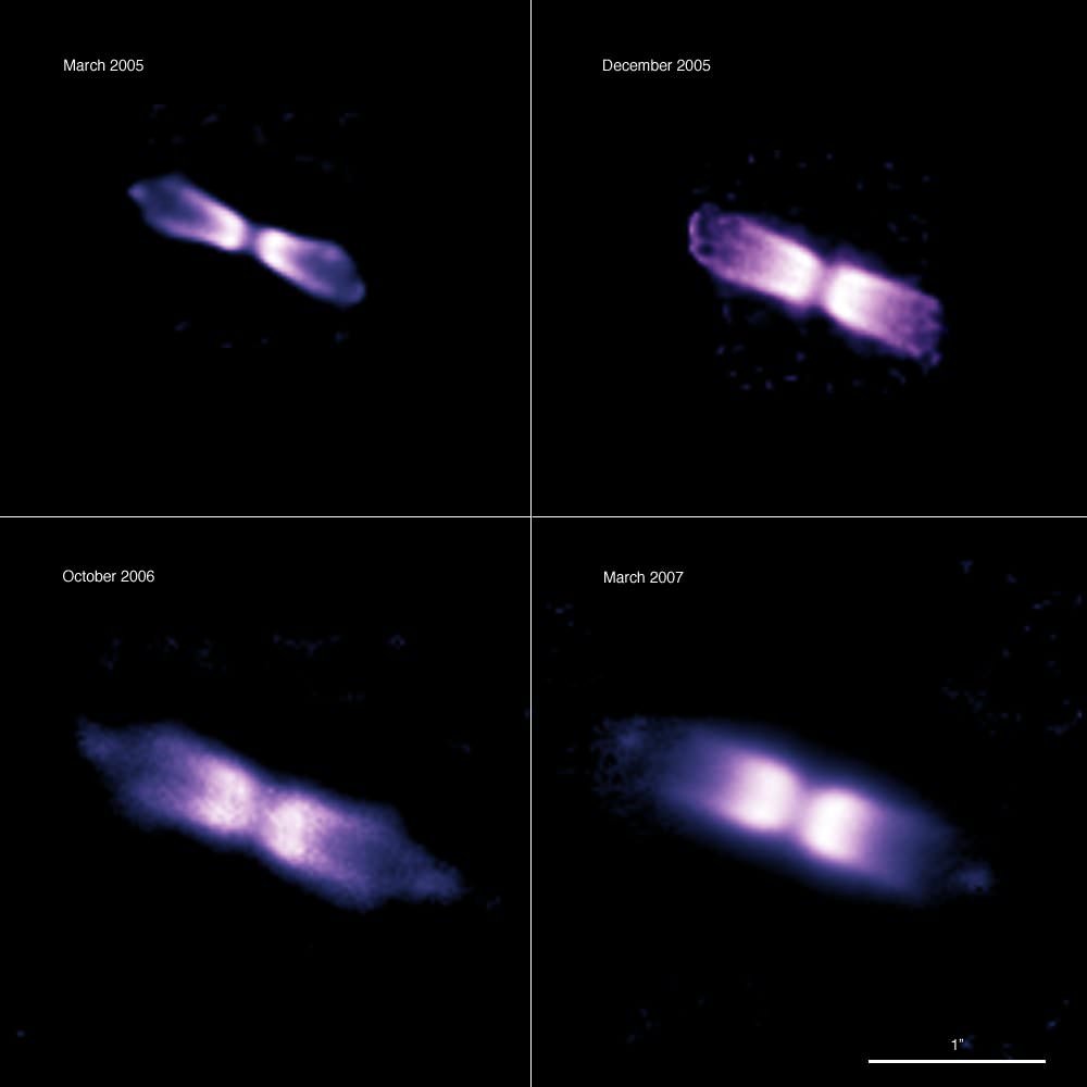
The 2009 paper by Woudt, Steeghs, and Karowska that Nancy cited, suggested accretion might continue until the white dwarf passed the Chandrasekhar limit and exploded as a type Ia supernova. However, the authors of the new paper, led by V. P. Goranskij at Moscow University, say that this 2000 detonation has effectively ruled out that possibility because an explosion of that magnitude would likely destroy the envelope of the donor star. Their evidence for this is the very same structure Woudt noted in his paper (shown above).
While the structure looks to be bipolar in nature, other observations have suggested that there is an additional component along the line of sight and that the structure is more of a doughnut shape. In this case, the total amount of material lost is higher than originally anticipated and must have come from from the envelope of the companion star. Additionally, observations in wavelengths able to pierce the dust have been unable to resolve a strong stellar source which suggests that the donor star’s envelope has been largely blown away as well. Additionally, this large and rapid loss of mass from the system may have broken the gravitational bond between the two stars and allowed the giant star to be ejected from the system, which would also preclude the possibility of a supernova in the future.
The conclusion is that V445 Puppis is not a candidate for a supernova of any type in the future. It’s own premature fireworks have likely destroyed whatever chance it may have had for an even grander show in the future.