[/caption]
With the recent milestone of the discovery of the 500th extra solar planet the future of planetary astronomy is promising. As the number of known planets increases so does our knowledge. With the addition of observations of atmospheres of transiting planets, astronomers are gaining a fuller picture of how planets form and live.
Thus far, the observations of atmospheres have been limited to the “Hot-Jupiter” type of planets which often puff up, extending their atmospheres and making them easier to observe. However, a recent set of observations, to be published in the December 2nd issue of Nature, have pushed the lower limit and extended observations of exoplanetary atmospheres to a super-Earth.
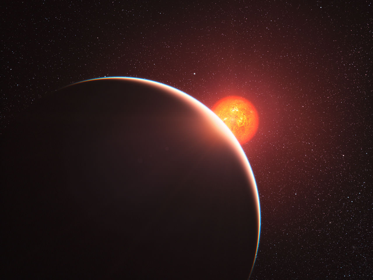
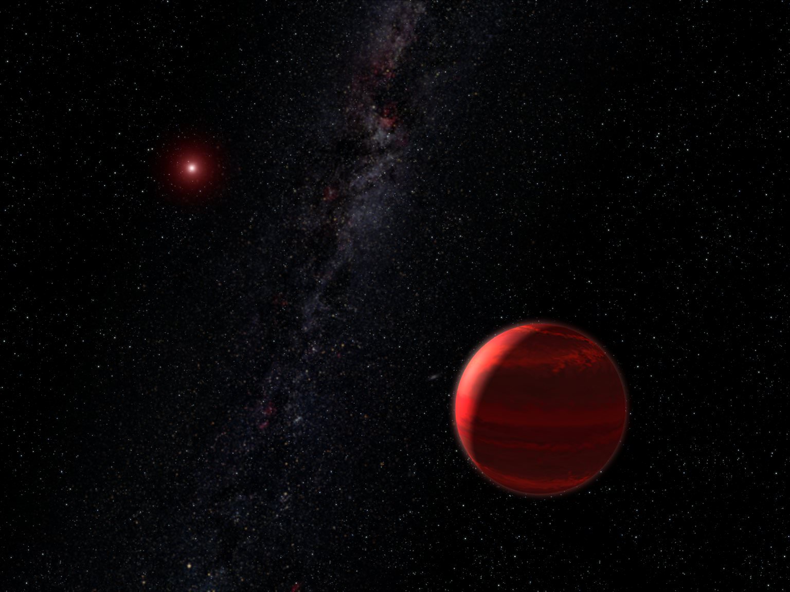
The planet in question, GJ 1214b passes in front of its parent star when viewed from Earth allowing for minor eclipses which help astronomers determine features of the system such as its radius and also its density. Earlier work, published in the Astrophysical Journal in August of this year, noted that the planet had an unusually low density (1.87 g/cm3). This ruled out an entirely rocky or iron based planet as well as even a giant snowball composed entirely of water ice. The conclusion was that the planet was surrounded by a thick gaseous atmosphere and the three possible atmospheres were proposed that could satisfy the observations.
The first was that the atmosphere was accreted directly from the protoplanetary nebula during formation. In this instance, the atmosphere would likely retain much of the primordial composition of hydrogen and helium since the mass would be sufficient to keep it from escaping readily. The second was that the planet itself is composed mostly of ices of water, carbon dioxide, carbon monoxide and other compounds. If such a planet formed, sublimation could result in the formation of an atmosphere that would be unable to escape. Lastly, if a strong component of rocky material formed the planet, outgassings could produce an atmosphere of water steam from geysers, as well as carbon monoxide and carbon dioxide and other gasses.
The challenge for following astronomers would be to match the spectra of the atmosphere to one of these models, or possibly a new one. The new team is composed of Jacob Bean, Eliza Kempton, and Derek Homeier, working from the University of Göttingen and the University of California, Santa Cruz. Their spectra of the planet’s atmosphere was largely featureless, showing no strong absorption lines. This largely rules out the first of the cases in which the atmosphere is mostly hydrogen unless there is a thick layer of clouds obscuring the signal from it. However, the team notes that this finding is consistent with an atmosphere composed largely of vapors from ices. The authors are careful to note that “the planet would not harbor any liquid water due to the high temperatures present throughout its atmosphere.”
These findings don’t conclusively demonstrate that nature of the atmosphere, but narrow down the degeneracy to either a steam filled atmosphere or one with thick clouds and haze. Despite not completely narrowing down the possibilities, Bean notes that the application of transit spectroscopy to a super-Earth has “reached a real milestone on the road toward characterizing these worlds.” For further study, Bean suggests that “[f]ollow-up observations in longer wavelength infrared light are now needed to determine which of these atmospheres exists on GJ 1214b.”
 for Universe Today")