Universe Today

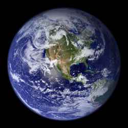
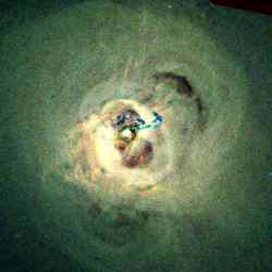
Artist’s impression of Earth auroras. Image credit: NASA Click to enlarge
Scientists from NASA and the National Science Foundation discovered a way to combine ground and space observations to create an unprecedented view of upper atmosphere disturbances during space storms.

Large, global-scale disturbances resemble weather cold fronts. They form in the Earth’s electrified upper atmosphere during space storms. The disturbances result from plumes of electrified plasma that form in the ionosphere. When the plasma plumes pass overhead, they impede low and high frequency radio communications and delay Global Positioning System navigation signals.

“Previously, they seemed like random events,” said John Foster, associate director of the Massachusetts Institute of Technology’s Haystack Observatory. He is principal investigator of the Foundation supported Millstone Hill Observatory, Wesford, Mass.

“People knew there was a space storm that must have disrupted their system, but they had no idea why,” said Tony Mannucci, group supervisor of Ionospheric and Atmospheric Remote Sensing at NASA’s Jet Propulsion Laboratory, Pasadena, Calif. “Now we know it’s not just chaos; there is cause and effect. We are beginning to put together the full picture, which will ultimately let us predict space storms.”

Predicting space weather is a primary goal of the National Space Weather Program involving NASA, the foundation and several other federal agencies. The view researchers created allowed them to link movement of the plumes to processes that release plasma into space. “Discovering this link is like discovering the movement of cold fronts is responsible for sudden thunderstorms,” said Jerry Goldstein, principal scientist at the Southwest Research Institute, San Antonio.

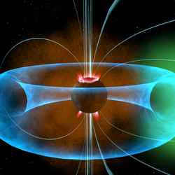
Since the occurrence of plasma plumes in the ionosphere disrupts GPS signals, they provide a continuous monitor of these disturbances. Researchers discovered a link between GPS data and satellite images of the plasmasphere. The plasmasphere is a plasma cloud surrounding Earth above the ionosphere. It is being observed from NASA’s Imager for Magnetopause to Aurora Global Exploration satellite. The researchers discovered the motion of the ionospheric plumes corresponded to the ejection of plasma from the plasmasphere during space storms.

The combined observations allowed construction of an underlying picture of the processes during space storms, when the Earth’s magnetic field is buffeted by hot plasma from the sun. As the solar plasma blows by, it generates an electric field that is transmitted to the plasmasphere and ionosphere. This electric field propels the ionospheric and the plasmaspheric plasma out into space. For the first time, scientists can directly connect the plasma observed in the ionosphere with the plasmasphere plumes that extend many thousand of kilometers into space.

“We also know these disturbances occur most often between noon and dusk, and between mid to high latitudes, due to the global structure of the electric and magnetic fields during space storms,” said Anthea Coster of the Haystack Observatory. “Ground and space based, and in situ measurements are allowing scientists to understand the ionosphere-thermosphere-magnetosphere as a coupled system.”

The plumes degrade GPS signals in two primary ways. First, they cause position error by time delaying the propagation of GPS signals. Second, the turbulence they generate causes receivers to lose the signal through an effect known as scintillation. It is similar to the apparent twinkling of stars caused by atmospheric turbulence.

Researchers are presenting the findings today during the American Geophysical Union meeting in San Francisco, Calif. For information about space weather and other research on the Web, visit:
http://www.nasa.gov/vision/universe/solarsystem/cold_front.html

Original Source: NASA News Release

Earth. Image credit: NASA Click to enlarge
The history of life on Earth is closely linked to the appearance of oxygen in the atmosphere. The current scientific consensus holds that significant amounts of oxygen first appeared in Earth’s atmosphere some 2.4 billion years ago, with a second large increase in atmospheric oxygen occurring much later, perhaps around 600 million years ago.

However, new findings by University of Maryland geologists suggest that the second jump in atmospheric oxygen actually may have begun much earlier and occurred more gradually than previously thought. The findings were made possible using a new tool for tracking microbial life in ancient environments developed at Maryland. Funded by the National Science Foundation and NASA, the work appears in the December 2 issue of Science.

Graduate researcher David Johnston, research scientist Boswell Wing and colleagues in the University of Maryland’s department of geology and Earth System Science Interdisciplinary Center led an international team of researchers that used high-precision measurements of a rare sulfur isotope, 33S, to establish that ancient marine microbes known as sulfur disproportionating prokaryotes were widely active almost 500 million years earlier than previously thought.

The intermediate sulfur compounds used by these sulfur disproportionating bacteria are formed by the exposure of sulfide minerals to oxygen gas. Thus, evidence of widespread activity by this type of bacteria has been interpreted by scientists as evidence of increased atmospheric oxygen content.

“These measurements imply that sulfur compound disproportionation was an active part of the sulfur cycle by [1.3 million years ago], and that progressive Earth surface oxygenation may have characterized the [middle Proterozoic],” the authors write.

The Proterozoic is the period in Earth’s history from about 2.4 billion years ago to 545 million years ago.

“The findings also demonstrate that the new 33S-based research method can be used to uniquely track the presence and character of microbial life in ancient environments and provide a glimpse of evolution in action,” said Johnston. “This approach provides a significant new tool in the astrobiological search for early life on Earth and beyond.”

The Air That We Breathe

When our planet formed some 4.5 billion years ago, virtually all the oxygen on Earth was chemically bound to other elements. It was in solid compounds like quartz and other silicate minerals, in liquid compounds like water, and in gaseous compounds like sulfur dioxide and carbon dioxide. Free oxygen — the gas that allows us to breath, and which is essential to all advanced life — was practically non-existent.

Scientists have long thought that appearance of oxygen in the atmosphere was marked by two distinct jumps in oxygen levels. In recent years, researchers have used a method developed by University of Maryland geologist James Farquhar and Maryland colleagues to conclusively determine that significant amounts of oxygen first appeared in Earth’s atmosphere some 2.4 billion years ago. Sometimes referred to as the “Great Oxidation Event,” this increase marks the beginning of the Proterozoic period.

A general scientific consensus has also held that the second major rise in atmospheric oxygen occurred some 600 million years ago, with oxygen rising to near modern levels at that time. Evidence of multicellular animals first appears in the geologic around this time.

“There has been a lot of discussion about whether the second major increase in atmospheric oxygen was quick and stepwise, or slow and progressive,” said Wing. “Our results support the idea that the second rise was progressive and began around 1.3 billion years ago, rather than 0.6 billion years ago.”

In addition to Johnston, Wing’s Maryland co-authors on the Dec. 2 paper are geology colleagues James Farquhar and Jay Kaufman. Their group works to document links between sulfur isotopes and the evolution of Earth’s atmosphere using a combination of field research, laboratory analysis of rock samples, geochemical models, photochemical experiments with sulfur-bearing gases and microbial experiments.

“Active microbial sulfur disproportionation in the Mesoproterozoic” by David T. Johnston, Boswell A. Wing, James Farquhar and Alan J. Kaufman, University of Maryland; Harald Strauss, Universit?t M?nster; Timothy W. Lyons, University of California, Riverside; Linda C. Kah, University of Tennessee; Donald E. Canfield, Southern Denmark University: Science, Dec. 2, 2005.

Original Source: UM News Release