Take a peek inside Blue Origin's New Shepard crew capsule. Credit: Blue Origin.
Blue Origin founder Jeff Bezos provided a sneak peek today into the interior of the New Shepard crew capsule, the suborbital vehicle for space tourism. He released a few images which illustrate what the flight experience might be like on board.
“Our New Shepard flight test program is focused on demonstrating the performance and robustness of the system,” Bezos said via an email release. “In parallel, we’ve been designing the capsule interior with an eye toward precision engineering, safety, and comfort.”
Take a look:
A view of the interior of the New Shepard crew capsule from Blue Origin. Credit: Blue Origin.
The interior has six seats with large windows for a great view of our planet.
“Every seat’s a window seat,” Bezos said.
What looks like a console in the center of the capsule is actually the escape motor to protect future passengers from any anomaly during launch. Unlike the Apollo escape system that used an escape “tower” motor located on top of the capsule to ‘pull’ the crew cabin away from a failing booster, New Shepard’s escape system is mounted underneath the capsule, to ‘push’ the capsule away from a potentially exploding booster. Blue Origin successfully tried out this escapes motor in October 2016 during an in-flight test.
Blue Origin touts the view from the New Shepard crew capsule as ‘the largest windows ever in space.’ Credit: Blue Origin.
Blue Origin’s suborbital rocket is named after Alan Shepard, the first NASA astronaut to take a suborbital trip to space in 1961. Their orbital rocket will be named New Glenn, named for John Glenn, the first American in orbit. Blue Origin is also developing a larger rocket to bring payloads beyond Earth orbit, and they’ve named that vehicle after Neil Armstrong, the first human to walk on the Moon.
Blue Origin hasn’t released a timeline yet of when they will be flying their first paying passengers; all Bezos has said is that he hopes to fly as soon as possible.
The commercial company describes the experience this way:
Following a thrilling launch, you’ll soar over 100 km above Earth—beyond the internationally recognized edge of space. You’ll help extend the legacy of space explorers who have come before you, while pioneering access to the space frontier for all.
Sitting atop a 60-foot-tall rocket in a capsule designed for six people, you’ll feel the engine ignite and rumble under you as you climb through the atmosphere. Accelerating at more than 3 Gs to faster than Mach 3, you will count yourself as one of the few who have gone these speeds and crossed into space.
Blue Origin’s black feather logo on the New Shepard rocket is ‘a symbol of the perfection of flight,’ says founder Jeff Bezos. Credit: Blue Origin.
“We are building Blue Origin to seed an enduring human presence in space, to help us move beyond this blue planet that is the origin of all we know,” Bezos said in the press release after a successful test flight of the New Shepard rocket in 2015. “We are pursuing this vision patiently, step-by-step. Our fantastic team in Kent, Van Horn and Cape Canaveral is working hard not just to build space vehicles, but to bring closer the day when millions of people can live and work in space.”
Blue Origin’s black feather logo on the New Shepard rocket is ‘a symbol of the perfection of flight,’ says founder Jeff Bezos, and “flight with grace and power in its functionality and design.”
Their moto, “Gradatim Ferociter” is Latin for “Step by Step, Ferociously.” Bezos has said that is how they are approaching their goals in spaceflight.
Find out more about the Blue Origin “Astronaut Experience” on their website.
If you’re lucky enough to be attending the 33rd Space Symposium in Colorado Springs April 3-6, 2017, you can see the New Shepard capsule for yourself. “The high-fidelity capsule mockup will be on display alongside the New Shepard reusable booster that flew to space and returned five times.” Bezos said.
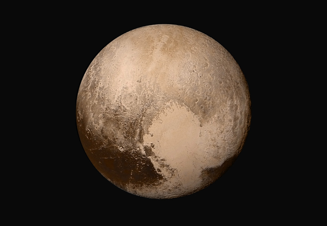
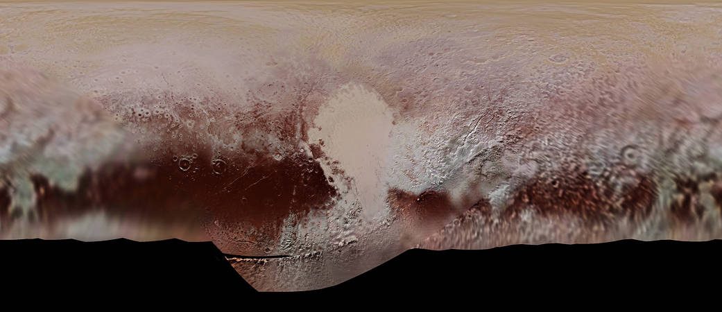
New Horizon's July 2015 flyby of Pluto captured this iconic image of the heart-shaped region called Tombaugh Regio. Credit:
NASA/JHUAPL/SwRI.
Discovered in 1930 by Clyde Tombaugh, Pluto was once thought to be the ninth and outermost planet of the Solar System. However, due to the formal definition adopted in 2006 at the 26th General Assembly of the International Astronomical Union (IAU), Pluto ceased being the ninth planet of the Solar System and has become alternately known as a “Dwarf Planet”, “Plutiod”, Trans-Neptunian Object (TNO) and Kuiper Belt Object (KBO).
Despite this change of designation, Pluto remains one of the most fascinating celestial bodies known to astronomers. In addition to having a very distant orbit around the Sun (and hence a very long orbital period) it also has the most eccentric orbit of any planet or minor planet in the Solar System. This makes for a rather long year on Pluto, which lasts the equivalent of 248 Earth years!
Orbital Period:
With an extreme eccentricity of 0.2488, Pluto’s distance from the Sun ranges from 4,436,820,000 km (2,756,912,133 mi) at perihelion to 7,375,930,000 km (4,583,190,418 mi) at aphelion. Meanwhile, it’s average distance (semi-major axis) from the Sun is 5,906,380,000 km (3,670,054,382 mi). Another way to look at it would be to say that it orbits the Sun at an average distance of 39.48 AU, ranging from 29.658 to 49.305 AU.
New Horizons trajectory and the orbits of Pluto and 2014 MU69.
At its closest, Pluto actually crosses Neptune’s orbit and gets closer to the Sun. This orbital pattern takes place once every 500 years, after which the two objects then return to their initial positions and the cycle repeats. Their orbits also place them in a 2:3 mean-motion resonance, which means that for every two orbits Pluto makes around the Sun, Neptune makes three.
The 2:3 resonance between the two bodies is highly stable, and is preserved over millions of years. The last time this cycle took place was between 1979 to 1999, when Neptune was farther from the Sun than Pluto. Pluto reached perihelion in this cycle – i.e. its closest point to the Sun – on September 5th, 1989. Since 1999, Pluto returned to a position beyond that of Neptune, where it will remain for the following 228 years – i.e. until the year 2227.
Sidereal and Solar Day:
Much like the other bodies in our Solar System, Pluto also rotates on its axis. The time it takes for it to complete a single rotation on its axis is known as a “Sidereal Day”, while the amount of time it takes for the Sun to reach the same point in the sky is known as a “Solar Day”. But due to Pluto’s very long orbital period, a sidereal day and a solar day on Pluto are about the same – 6.4 Earth days (or 6 days, 9 hours, and 36 minutes).
View from the surface of Pluto, showing its large moon Charon in the distance. Credit: New York Time
It is also worth noting that Pluto and Charon (its largest moon) are actually more akin to a binary system rather than a planet-moon system. This means that the two worlds orbit each other, and that Charon is tidally locked around Pluto. In other words, Charon takes 6 days and 9 hours to orbit around Pluto – the same amount of time it takes for a day on Pluto. This also means that Charon is always in the same place in the sky when seen from Pluto.
In short, a single day on Pluto lasts the equivalent of about six and a half Earth days. A year on Pluto, meanwhile, lasts the equivalent of 248 Earth years, or 90,560 Earth days! And for the entire year, the moon is hanging overhead and looming large in the sky. But factor in Pluto’s axial tilt, and you will come to see just how odd an average year on Pluto is.
Seasonal Change:
It has been estimated that for someone standing on the surface of Pluto, the Sun would appear about 1,000 times dimmer than it appears from Earth. So while the Sun would still be the brightest object in the sky, it would look more like a very bright star that a big yellow disk. But despite being very far from the Sun at any given time, Pluto’s eccentric orbit still results in some considerable seasonal variations.
On the whole, the surface temperature of Pluto does not change much. It’s surface temperatures are estimated to range from a low of 33 K (-240 °C; -400 °F ) to a high of 55 K (-218 °C; -360°F) – averaging at around 44 K (-229 °C; -380 °F). However, the amount of sunlight each side receives during the course of a year is vastly different.
Compared to most of the planets and their moons, the Pluto-Charon system is oriented perpendicular to its orbit. Much like Uranus, Pluto’s very high axial tilt (122 degrees) essentially means that it is orbiting on its side relative to its orbital plane. This means that at a solstice, one-quarter of Pluto’s surface experiences continuous daylight while the other experiences continuous darkness.
This is similar to what happens in the Arctic Circle, where the summer solstice is characterized by perpetual sunlight (i.e. the “Midnight Sun”) and the winter solstice by perpetual night (“Arctic Darkness”). But on Pluto, these phenomena affect nearly the entire planet, and the seasons last for close to a century.
Even if it is no longer considered a planet (though this could still change) Pluto still has some very fascinating quarks, all of which are just as worthy of study as those of the other eight planets. And the time it takes to complete a full year on Pluto, and all the seasonal changes it goes through, certainly rank among the top ten!
For more information, be sure to check out NASA’s Solar System Exploration page on Pluto, and the New Horizon’s mission page for information on Pluto’s seasons.
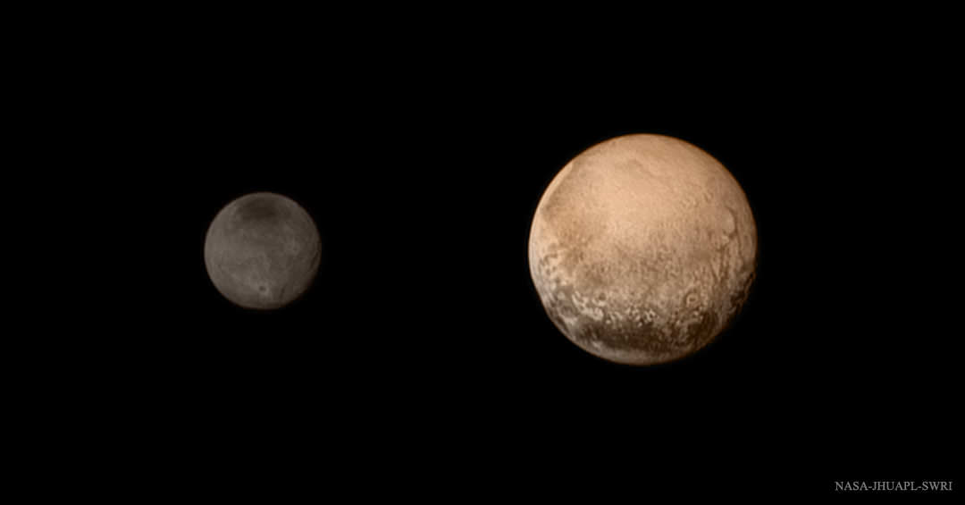
Pluto was re-classified as a dwarf planet based on our growing understanding of its nature. Will Schlaufman's new study help us more accurately classify gas giants and brown dwarfs? NASA's New Horizons spacecraft captured this high-resolution enhanced color view of Pluto on July 14, 2015. Credit: NASA/JHUAPL/SwRI
When Pluto was first discovered by Clybe Tombaugh in 1930, astronomers believed that they had found the ninth and outermost planet of the Solar System. In the decades that followed, what little we were able to learn about this distant world was the product of surveys conducted using Earth-based telescopes. Throughout this period, astronomers believed that Pluto was a dirty brown color.
In recent years, thanks to improved observations and the New Horizons mission, we have finally managed to obtain a clear picture of what Pluto looks like. In addition to information about its surface features, composition and tenuous atmosphere, much has been learned about Pluto’s appearance. Because of this, we now know that the one-time “ninth planet” of the Solar System is rich and varied in color.
Composition:
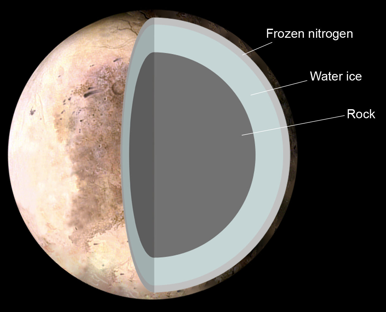
With a mean density of 1.87 g/cm3, Pluto’s composition is differentiated between an icy mantle and a rocky core. The surface is composed of more than 98% nitrogen ice, with traces of methane and carbon monoxide. Scientists also suspect that Pluto’s internal structure is differentiated, with the rocky material having settled into a dense core surrounded by a mantle of water ice.
The Theoretical structure of Pluto, consisting of 1. Frozen nitrogen 2. Water ice 3. Rock. Credit: NASA/Pat Rawlings
The diameter of the core is believed to be approximately 1700 km, which accounts for 70% of Pluto’s total diameter. Thanks to the decay of radioactive elements, it is possible that Pluto contains a subsurface ocean layer that is 100 to 180 km thick at the core–mantle boundary.
Pluto has a thin atmosphere consisting of nitrogen (N2), methane (CH4), and carbon monoxide (CO), which are in equilibrium with their ices on Pluto’s surface. However, the planet is so cold that during part of its orbit, the atmosphere congeals and falls to the surface. The average surface temperature is 44 K (-229 °C), ranging from 33 K (-240 °C) at aphelion to 55 K (-218 °C) at perihelion.
Appearance:
Pluto’s surface is very varied, with large differences in both brightness and color. Pluto’s surface also shows signs of heavy cratering, with ones on the dayside measuring 260 km (162 mi) in diameter. Tectonic features including scarps and troughs has also been seen in some areas, some as long as 600 km (370 miles).
Mountains have also been seen that are between 2 to 3 kilometers (6500 – 9800 ft) in elevation above their surroundings. Like much of the surface, these features are believed to be composed primarily of frozen nitrogen, carbon monoxide, and methane, which are believed to sit atop a “bedrock” of frozen water ice.
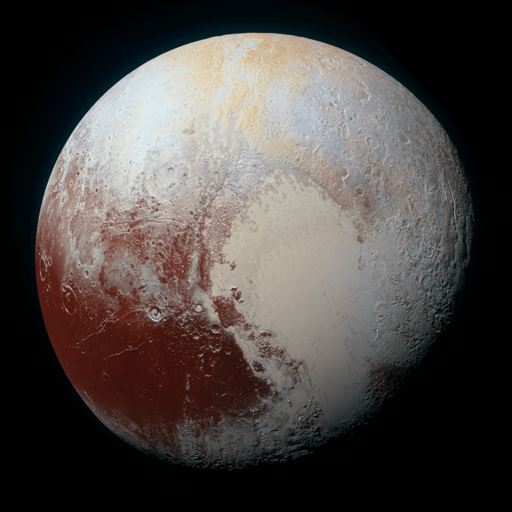
Color mosaic map of Pluto’s surface, created from the New Horizons many photographs. Credit: NASA/JHUAPL/SwRI
The surface also has many dark, reddish patches due to the presence of tholins, which are created by charged particles from the Sun interacting with mixtures of methane and nitrogen. Pluto’s visual apparent magnitude averages 15.1, brightening to 13.65 at perihelion. In other words, the planet has a range of colors, including pale sections of off-white and light blue, to streaks of yellow and subtle orange, to large patches of deep red.
Overall, its appearance could be described as “ruddy”, given that the combination can lend it a somewhat brown and earthy appearance from a distance. In fact, prior to the New Horizon‘s mission, which provided the first high-resolution, close-up images of the planet, this is precisely what astronomers believed Pluto looked like.
Major Surface Features:
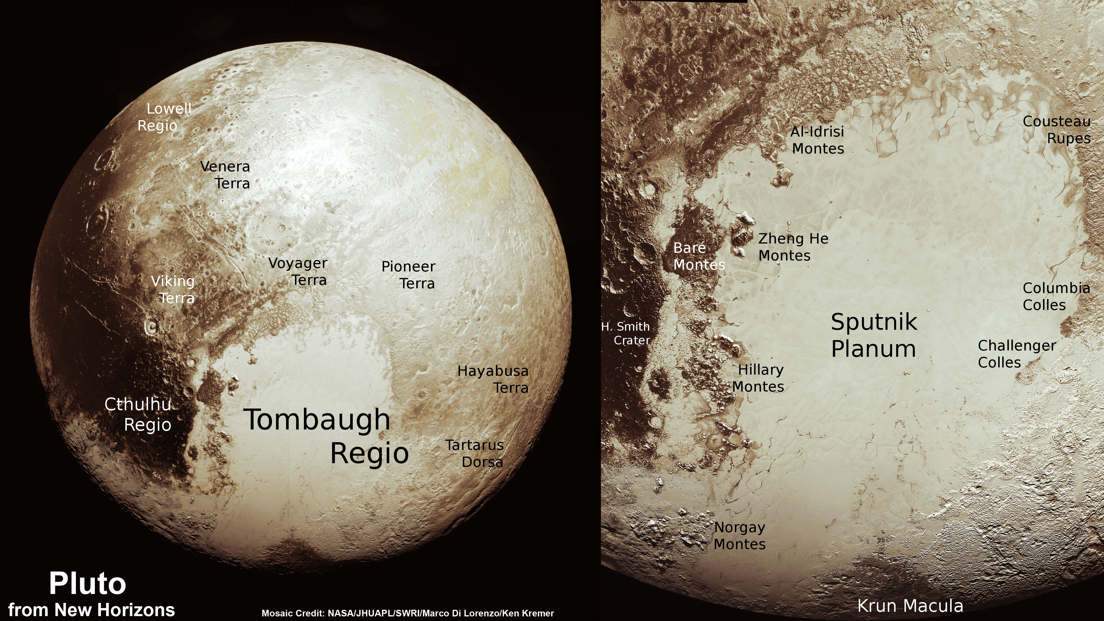
Several different regions (“regio”) have been characterized based on the notable features they possess. Perhaps the best known is the large, pale area nicknamed the “Heart” – aka. Tombaugh Regio (named after Pluto’s founder). This large bright area is located on the side of Pluto that lies opposite the side that faces Charon, and is named because of its distinctive shape.
Tombaugh Regio is about 1,590 km (990 mi) across and contains 3,400 m (11,000 ft) mountains made of water ice along its southwestern edge. The lack of craters suggests that its surface is relatively young (about 100 million years old) and hints at Pluto being geologically active. The Heart can be subdivided into two lobes, which are distinct geological features that are both bright in appearance.
This new global mosaic view of Pluto was created from the latest high-resolution images to be downlinked from NASA’s New Horizons spacecraft and released on Sept. 11, 2015. Credits: NASA/Johns Hopkins APL/SwRI/Marco Di Lorenzo/Ken Kremer
The western lobe, Sputnik Planitia, is vast plain of nitrogen and carbon monoxide ices measuring 1000 km in width. It is divided into polygonal sections that are believed to be convection cells, which carry blocks of water ice and sublimation pits along towards the edge of the plain. This region is especially young (less than 10 million years old), which is indicated by its lack of cratering.
Then there is the large, dark area on the trailing hemisphere known as Cthulhu Regio (aka.the “Whale”). Named for its distinctive shape, this elongated, dark region along the equator is the largest dark feature on Pluto – measuring 2,990 km (1,860 mi) in length. The dark color is believed to be the result methane and nitrogen in the atmosphere interacting with ultraviolet light and cosmic rays, creating the dark particles (“tholins”) common to Pluto.
And then there are the “Brass Knuckles”, a series of equatorial dark areas on the leading hemisphere. These features average around 480 km (300 mi) in diameter, and are located along the equator between the Heart and the tail of the Whale.
New Horizons Mission:
The NH mission launched from Cape Canaveral Air Force Station in Florida on January 19th, 2006. After swinging by Jupiter for a gravity boost and to conduct some scientific studies in February of 2007, it reached Pluto in the summer of 2015. Once there, it conducted a six month-long reconnaissance flyby of Pluto and its system of moons, culminating with a closest approach that occurred on July 14th, 2015.
A portrait from the final approach of the New Horizons spacecraft to the Pluto system on July 11th, 2015. Pluto and Charon display striking color and brightness contrast in this composite image. Credit: NASA-JHUAPL-SWRI.
The first images of Pluto acquired by NH were taken on September 21st to 24th, 2006, during a test of the Long Range Reconnaissance Imager (LORRI). At the time, the probe was still at a distance of approximately 4.2 billion km (2.6 billion mi) or 28 AU, and the photos were released on November 28th, 2006. Between July 1st and 3rd, the first images were taken that were able to resolved Pluto and its largest moon, Charon, as separate objects.
Between July 19th–24th, 2014, the probe snapped 12 images of Charon revolving around Pluto, covering almost one full rotation at distances ranging from 429 to 422 million kilometers (267,000,000 to 262,000,000 mi). After a brief hibernation during its final approach, New Horizons “woke up” on Dec. 7th, 2014. Distant-encounter operations began on January 4th, 2015, and NH began taking images of Pluto as it grew closer.
During its closest approach (July 14th, 2015, at at 11:50 UTC), the NH probe passed within 12,500 km (7,800 mi) of Pluto. About 3 days before making its closest approach, long-range imaging of Pluto and Charon took place that were 40 km (25 mi) in resolution, which allowed for all sides of both bodies to be mapped out.
Close-range imaging also took place twice a day during this time to search for any indication of surface changes. The NH probe also analyzed Pluto’s atmosphere using its suite of scientific instruments. This included it’s ultraviolet imaging spectrometer (aka. Alice) and the Radio Science EXperiment (REX), which analyzed the composition and structure of Pluto’s atmosphere.
Haze with multiple layers in the atmosphere of Pluto. Part of the plain Sputnik Planitia with nearby mountains is seen below. Photo by New Horizons, taken 15 min after the closest approach to Pluto. Credit: NASA/JHUAPL/SwRI
It’s Solar Wind Around Pluto (SWAP) and Pluto Energetic Particle Spectrometer Science Investigation (PEPSSI) examined the interaction of Pluto’s high atmosphere with solar wind. Pluto’s diameter was also resolved by measuring the disappearance and reappearance of the radio occultation signal as the probe flew by behind Pluto. And the gravitational tug on the probe were used to determine Pluto’s mass and mass distribution.
All of this information has helped astronomers to make the first detailed maps of Pluto, and led to numerous discoveries about Pluto’s structure, composition, and the kinds of forces that actively shape its surface. The mission also led to the first true images of what Pluto looks like up close, revealing its true colors, it’s famous “Heart” region, and the many other now-famous features.
When it comes to dealing with the cosmos, we humans like to couch things in familiar terms. When examining exoplanets, we classify them based on their similarities to the planets in our own Solar System – i.e. terrestrial, gas giant, Earth-size, Jupiter-sized, Neptune-sized, etc. And when measuring astronomical distances, we do much the same.
For instance, one of the most commonly used means of measuring distances across space is known as an Astronomical Unit (AU). Based on the distance between the Earth and the Sun, this unit allows astronomers to characterize the vast distances between the Solar planets and the Sun, and between extra-solar planets and their stars.
Definition:
According to the current astronomical convention, a single Astronomical Unit is equivalent to 149,597,870.7 kilometers (or 92,955,807 miles). However, this is the average distance between the Earth and the Sun, as that distance is subject to variation during Earth’s orbital period. In other words, the distance between the Earth and the Sun varies in the course of a single year.
Earth’s orbit around the Sun, showing its average distance (or 1 AU). Credit: Huritisho/Wikipedia Commons
During the course of a year, the Earth goes from distance of 147,095,000 km (91,401,000 mi) from the Sun at perihelion (its closest point) to 152,100,000 km (94,500,000 mi) at aphelion (its farthest point) – or from a distance of 0.983 AUs to 1.016 AUs.
History of Development:
The earliest recorded example of astronomers estimating the distance between the Earth and the Sun dates back to Classical Antiquity. In the 3rd century BCE work, On the Sizes and Distances of the Sun and Moon – which is attributed to Greek mathematician Aristarchus of Samos – the distance was estimated to be between 18 and 20 times the distance between the Earth and the Moon.
However, his contemporary Archimedes, in his 3rd century BCE work Sandreckoner, also claimed that Aristarchus of Samos placed the distance of 10,000 times the Earth’s radius. Depending on the values for either set of estimates, Aristarchus was off by a factor of about 2 (in the case of Earth’s radius) to 20 (the distance between the Earth and the Moon).
The oldest Chinese mathematical text – the 1st century BCE treatise known as Zhoubi Suanjing – also contains an estimate of the distance between the Earth and Sun. According to the anonymous treatise, the distance could be calculated by conducting geometric measurements of the length of noontime shadows created by objects spaced at specific distances. However, the calculations were based on the idea that the Earth was flat.
Illustration of the Ptolemaic geocentric conception of the Universe, by Bartolomeu Velho (?-1568), from his work Cosmographia, made in France, 1568. Credit: Bibilotèque nationale de France, Paris
Famed 2nd century CE mathematician and astronomer Ptolemy relied on trigonometric calculations to come up with a distance estimate that was equivalent to 1210 times the radius of the Earth. Using records of lunar eclipses, he estimated the Moon’s apparent diameter, as well as the apparent diameter of the shadow cone of Earth traversed by the Moon during a lunar eclipse.
Using the Moon’s parallax, he also calculated the apparent sizes of the Sun and the Moon and concluded that the diameter of the Sun was equal to the diameter of the Moon when the latter was at it’s greatest distance from Earth. From this, Ptolemy arrived at a ratio of solar to lunar distance of approximately 19 to 1, the same figure derived by Aristarchus.
For the next thousand years, Ptolemy’s estimates of the Earth-Sun distance (much like most of his astronomical teachings) would remain canon among Medieval European and Islamic astronomers. It was not until the 17th century that astronomers began to reconsider and revise his calculations.
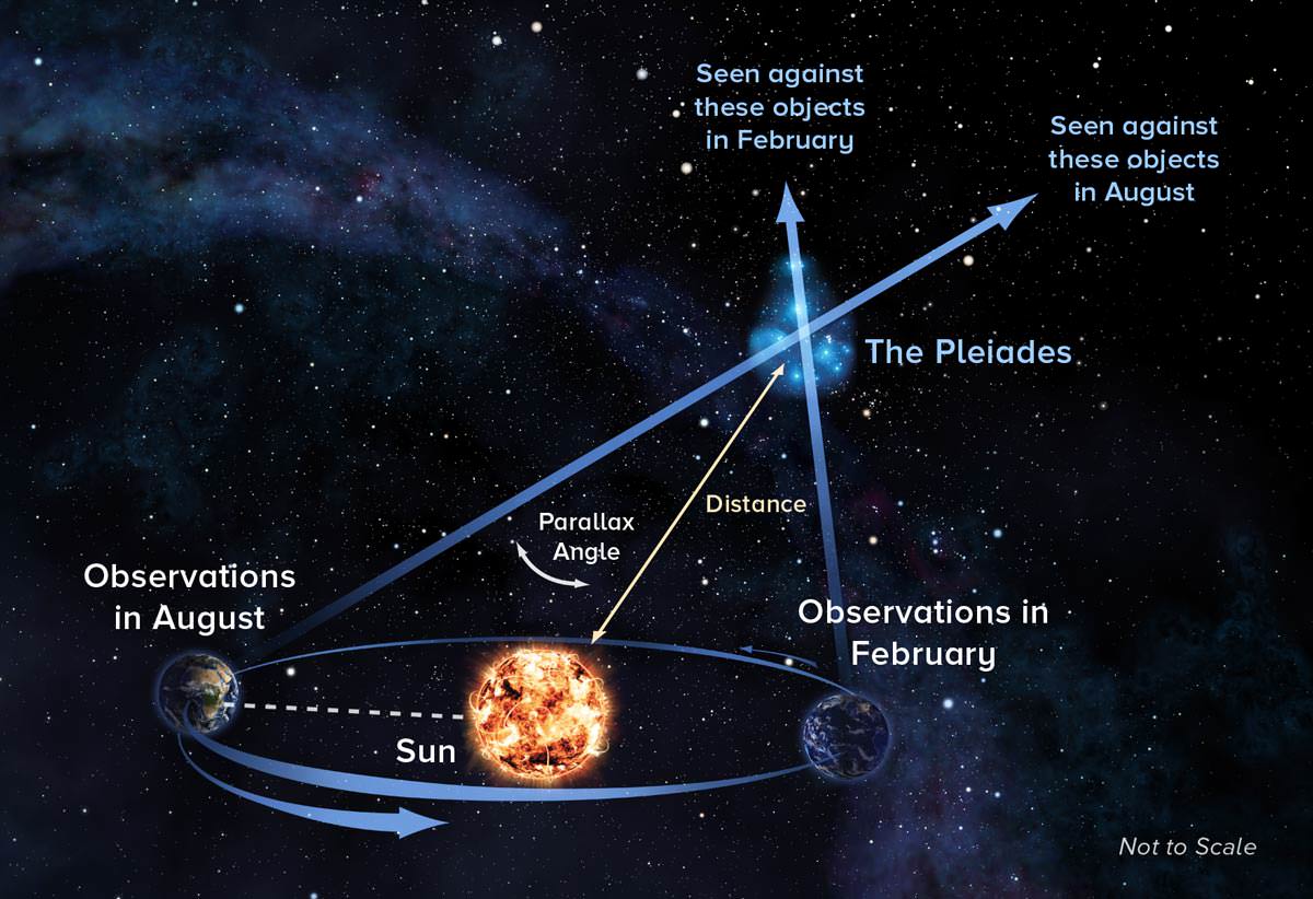
This was made possible thanks to the invention of the telescope, as well as Kepler’s Three Laws of Planetary Motion, which helped astronomers calculate the relative distances between the planets and the Sun with greater accuracy. By measuring the distance between Earth and the other Solar planets, astronomers were able to conduct parallax measurements to obtain more accurate values.
With parallax technique, astronomers observe object at opposite ends of Earth’s orbit around the Sun to precisely measure its distance. Credit: Alexandra Angelich, NRAO/AUI/NSF.
By the 19th century, determinations of about the speed of light and the constant of the aberration of light resulted in the first direct measurement of the Earth-Sun distance in kilometers. By 1903, the term “astronomical unit” came to be used for the first time. And throughout the 20th century, measurements became increasingly precise and sophisticated, thanks in part to accurate observations of the effects of Einstein’s Theory of Relativity.
Modern Usage:
By the 1960s, the development of direct radar measurements, telemetry, and the exploration of the Solar System with space probes led to precise measurements of the positions of the inner planets and other objects. In 1976, the International Astronomical Union (IAU) adopted a new definition during their 16th General Assembly. As part of their System of Astronomical Constants, the new definition stated:
“The astronomical unit of length is that length (A) for which the Gaussian gravitational constant (k) takes the value 0.01720209895 when the units of measurement are the astronomical units of length, mass and time. The dimensions of k² are those of the constant of gravitation (G), i.e., L³M-1T–2. The term “unit distance” is also used for the length A.”
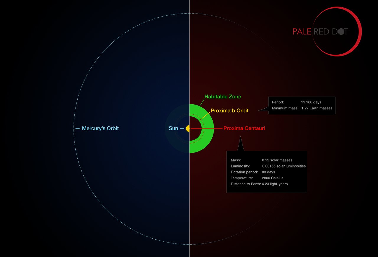
Infographic comparing the orbit of the planet around Proxima Centauri (Proxima b) with the same region of the Solar System. Credit: ESO
However, by 2012, the IAU determined that the equalization of relativity made the measurement of AUs too complex, and redefined the astronomical unit in terms of meters. In accordance with this, a single AU is equal to 149597870.7 km exactly (92.955807 million miles), 499 light-seconds, 4.8481368×10⁻⁶ of a parsec, or 15.812507×10⁻⁶ of a light-year.
Today, the AU is used commonly to measure distances and create numerical models for the Solar System. It is also used when measuring extra-solar systems, calculating the extent of protoplanetary clouds or the distance between extra-solar planets and their parent star. When measuring interstellar distances, AUs are too small to offer convenient measurements. As such, other units – such as the parsec and the light year – are relied upon.
The Universe is a huge place, and measuring even our small corner of it producing some staggering results. But as always, we prefer to express them in ways that are as relatable and familiar.
SpaceX conducts successful static hot fire test of 1st previously flown Falcon 9 booster atop Launch Complex 39A at the Kennedy Space Center on 27 Mar. 2017 as seen from Space View Park, Titusville, FL. History making launch of first recycled rocket is slated for 30 March 2017 with SES-10 telecommunications comsat. Credit: Ken Kremer/Kenkremer.com
SpaceX conducts successful static hot fire test of 1st previously flown Falcon 9 booster atop Launch Complex 39A at the Kennedy Space Center on 27 Mar. 2017 as seen from Space View Park, Titusville, FL. History making launch of first recycled rocket is slated for 30 March 2017 with SES-10 telecommunications comsat. Credit: Ken Kremer/Kenkremer.com
SPACE VIEW PARK/KENNEDY SPACE CENTER, FL – This afternoons (Mar. 27) successful hotfire test of a recycled Falcon 9 booster at the Kennedy Space Center sets SpaceX on course for a rendezvous with history involving the first ever relaunch of a ‘Flight-Proven’ rocket later this week.
The milestone mission to refly the first ever ‘used rocket’ is slated for lift off on Thursday, March 30, at 6 p.m. EDT from seaside Launch Complex 39A at NASA’s Kennedy Space Center in Florida, carrying the SES-10 telecommunications payload.
“Static fire test complete,” SpaceX confirmed via social media.
“Targeting Thursday, March 30 for Falcon 9 launch of SES-10.”
SES-10 is to be the first satellite launching on a SpaceX flight-proven rocket, gushes telecommunications giant SES.
The flight proven SpaceX Falcon 9 rocket will deliver SES-10 to a Geostationary Transfer Orbit (GTO).
The Falcon 9 booster to be recycled was initially launched in April 2016 for NASA on the SpaceX Dragon CRS-8 resupply mission to the International Space Station (ISS) under contract for the space agency.
The Falcon 9 first stage was recovered about 8 and a half minutes after liftoff via a propulsive soft landing on an ocean going droneship in the Atlantic Ocean some 400 miles (600 km) off the US East coast.
The brief engine test lasting approximately three seconds took place at 2 p.m. today, Monday March 27, with the sudden eruption of smoke and ash rushing into the air over historic pad 39A on NASA’s Kennedy Space Center during a picture perfect sunny afternoon – as I witnessed from Space View Park in Titusville, FL.
During today’s static fire test, the rocket’s first and second stages are fueled with liquid oxygen and RP-1 propellants like an actual launch, and a simulated countdown is carried out to the point of a brief engine ignition.
The hold down engine test with the erected rocket involved the ignition of all nine Merlin 1D first stage engines generating some 1.7 million pounds of thrust at pad 39A while the two stage rocket was restrained on the pad.
This is only the third Falcon 9 static fire test ever conducted on Pad 39A.
Pad 39A has been repurposed by SpaceX from its days as a NASA shuttle launch pad.
Watch this video of the March 27 static fire test from colleague Jeff Seibert:
Video Caption: SpaceX Falcon 9 hot fire test on March 27, 2017 for SES-10 launch on March 30 on KSC Pad 39A. Credit: Jeff Seibert
Space View Park is a great place to watch rocket launches from as it offers an unobstructed view across the inland river to the Kennedy Space Center and Cape Canaveral Air Force Station launch pads dotting the Florida Space Coast.
SpaceX, founded by billionaire and CEO Elon Musk, inked a deal in August 2016 with telecommunications giant SES, to refly a ‘Flight-Proven’ Falcon 9 booster.
Luxembourg-based SES and Hawthrone, CA-based SpaceX jointly announced the agreement to “launch SES-10 on a flight-proven Falcon 9 orbital rocket booster.”
Exactly how much money SES will save by utilizing a recycled rocket is not known. But SpaceX officials have been quoted as saying the savings could be between 10 to 30 percent.
This critical engine test opens the door to what will be only the third blastoff of the SpaceX commercial Falcon 9 rocket from seaside Launch Complex 39A at NASA’s Kennedy Space Center in Florida.
So SpaceX is definitely picking up the pace of launch operations as this blastoff comes barely 2 weeks after the prior launch on March 16 with EchoStar XXIII.
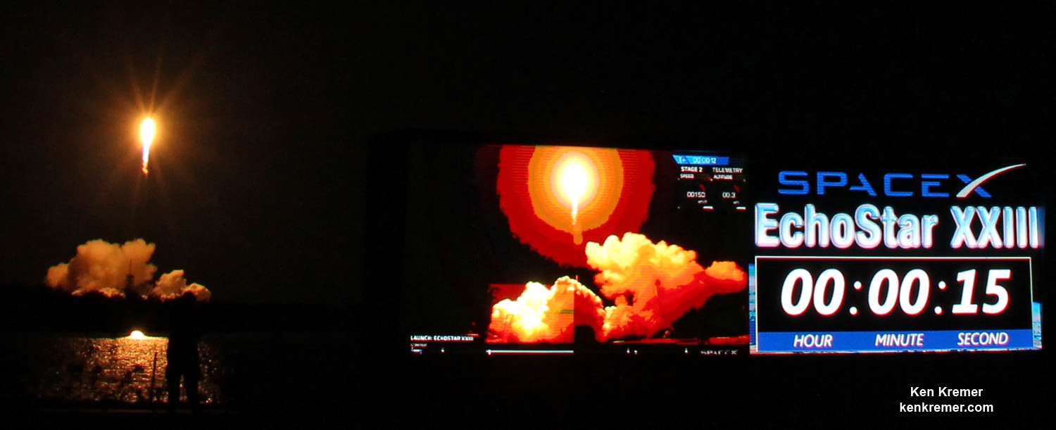
The SpaceX Falcon 9 launches the EchoStar 23 telecomsat from historic Launch Complex 39A with countdown clock in foreground at NASA’s Kennedy Space Center as display shows liftoff progress to geosynchronous orbit after post midnight blastoff on March 16 at 2:oo a.m. EDT. Credit: Ken Kremer/Kenkremer.com
Liftoff of the Falcon 9 carrying the SES-10 telecommunications satellite is now slated for 6 p.m. EDT at the opening of the launch window
The two and a half hour launch window closes at 8:30 p.m. EDT.
SES-10 will replace AMC-3 and AMC-4 to provide enhanced coverage and significant capacity expansion over Latin America, says SES.
“The satellite will be positioned at 67 degrees West, pursuant to an agreement with the Andean Community (Bolivia, Colombia, Ecuador and Peru), and will be used for the Simón Bolivar 2 satellite network.”
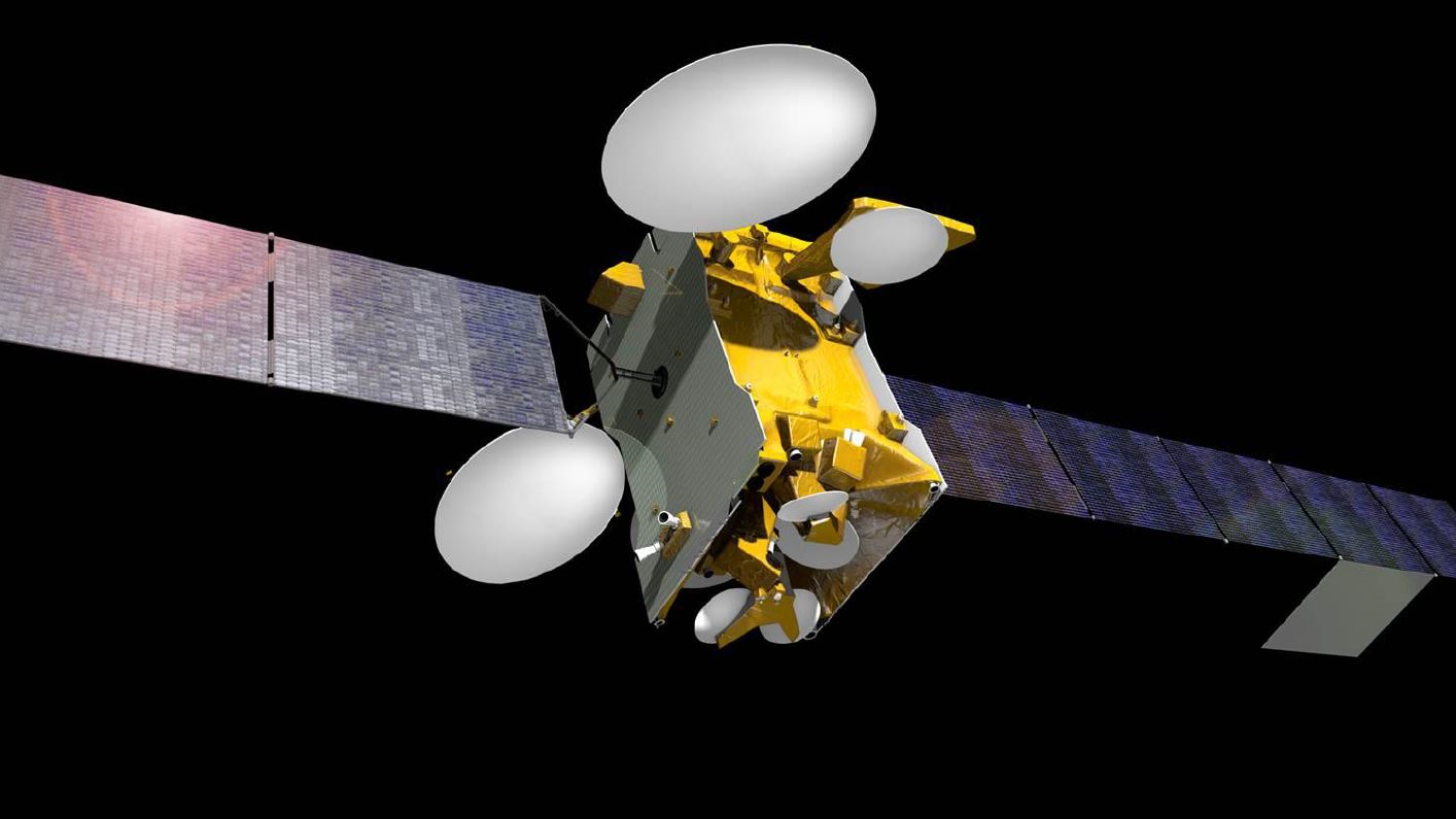
SES-10 satellite mission artwork. Credit: SES
Stay tuned here for Ken’s continuing Earth and Planetary science and human spaceflight news.
Learn more about SpaceX SES-10, EchoStar 23 and CRS-10 launches to ISS, ULA SBIRS GEO 3 launch, GOES-R launch, Heroes and Legends at KSCVC, OSIRIS-REx, InSight Mars lander, Juno at Jupiter, SpaceX AMOS-6, ISS, ULA Atlas and Delta rockets, Orbital ATK Cygnus, Boeing, Space Taxis, Mars rovers, Orion, SLS, Antares, NASA missions and more at Ken’s upcoming outreach events at Kennedy Space Center Quality Inn, Titusville, FL:
Mar 29/31, Apr 1: “SpaceX SES-10, EchoStar 23, CRS-10 launch to ISS, ULA Atlas SBIRS GEO 3 launch, GOES-R weather satellite launch, OSIRIS-Rex, SpaceX and Orbital ATK missions to the ISS, Juno at Jupiter, ULA Delta 4 Heavy spy satellite, SLS, Orion, Commercial crew, Curiosity explores Mars, Pluto and more,” Kennedy Space Center Quality Inn, Titusville, FL, evenings
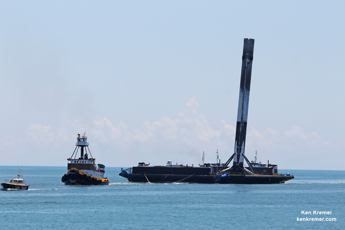
SpaceX Falcon 9 booster from Thaicom-8 launch on May 27, 2016 arrives at mouth of Port Canaveral, FL on June 2, 2016. Credit: Ken Kremer/kenkremer.com
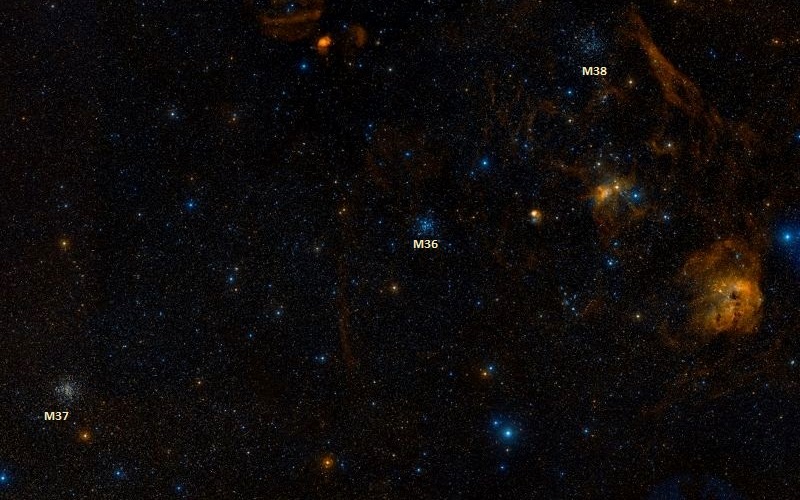
The open star cluster Messier 38, in proximity to Messier 36 and Messier 37. Credit: Wikisky
Welcome back to Messier Monday! In our ongoing tribute to the great Tammy Plotner, we take a look at the Starfish Cluster, otherwise known as Messier 38. Enjoy!
During the 18th century, famed French astronomer Charles Messier noted the presence of several “nebulous objects” in the night sky. Having originally mistaken them for comets, he began compiling a list of them so that others would not make the same mistake he did. In time, this list (known as the Messier Catalog) would come to include 100 of the most fabulous objects in the night sky.
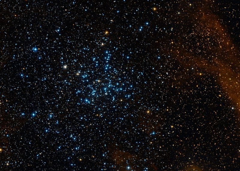
One of these objects it the Starfish Cluster, also known as Messier 38 (or M38). This open star cluster is located in the direction of the northern Auriga constellation, along with the open star clusters M36 and M37. While not the brightest of the three, the location of the Starfish within the polygon formed by the brightest stars of Auriga makes it very easy to find.
Description:
Cruising around our Milky Way some 4200 light years from our solar system, this 220 million year old group of stars spreads itself across about 25 light years of space. If you’re using a telescope, you may have noticed its not alone… Messier 38 might very well be a binary star cluster! As Anil K. Pandey (et al) explained in a 2006 study:
“We present CCD photometry in a wide field around two open clusters, NGC 1912 and NGC 1907. The stellar surface density profiles indicate that the radii of the clusters NGC 1912 and NGC 1907 are 14′ and 6′ respectively. The core of the cluster NGC 1907 is found to be 1′.6±0′.3, whereas the core of the cluster NGC 1912 could not be defined due to its significant variation with the limiting magnitude. The clusters are situated at distances of 1400±100 pc (NGC 1912) and 1760±100 pc (NGC 1907), indicating that in spite of their close locations on the sky they may be formed in different parts of the Galaxy.”
The Starfish Cluster also known as Messier 38. Credit: Wikisky
So what’s happening here? Chances are, when you’re looking at M38, you’re looking at a star cluster that’s currently undergoing a real close encounter! Said M.R. de Oliveira (et al) said in their 2002 study:
“The possible physical relation between the closely projected open clusters NGC 1912 (M 38) and NGC 1907 is investigated. Previous studies suggested a physical pair based on similar distances, and the present study explores in more detail the possible interaction. Spatial velocities are derived from available radial velocities and proper motions, and the past orbital motions of the clusters are retrieved in a Galactic potential model. Detailed N-body simulations of their approach suggest that the clusters were born in different regions of the Galaxy and presently experience a fly-by.”
However, it was Sang Hyun Lee and See-Woo Lee who gave us the estimates of M38’s distance and age. As they wrote in their 1996 study, “UBV CCD Photometry of Open Cluster NGC 1907 and NGC 1912“: “The distance difference of the two clusters is 300pc and the age difference is 150 Myr. These results imply that the two clusters are not physically connected.”
So, how do we know they are two clusters passing in the night? The credit for that goes to de Oliveira and colleagues, who also asserted in their 2002 study:
“These simulations also shows that the faster the clusters approach the weaker the tidal debris in the bridge region, which explain why there is, apparently, no evidence of a material link between the clusters and why it should not be expected. It would be necessary to analyse deep wide field CCD photometry for a more conclusive result about the apparent absence of tidal link between the clusters.”
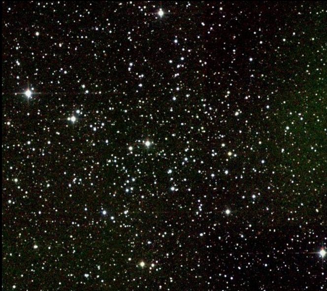
Atlas image mosaic of the Starfish Cluster (Messier 38), obtained as part of the Two Micron All Sky Survey (2MASS). Credit: NASA/NSF/Caltech/UofMass/IPAC
History of Observation:
This wonderful star cluster was originally discovered by Giovanni Batista Hodierna before 1654 and independently rediscovered by Le Gentil in 1749. However, it was Charles Messier’s catalog which brought it to attention:
“In the night of September 25 to 26, 1764, I have discovered a cluster of small stars in Auriga, near the star Sigma of that constellation, little distant from the two preceding clusters: this one is of square shape, and doesn’t contain any nebulosity, if one examines it with a good instrument: its extension may be 15 minutes of arc. I have determined its position: its right ascension was 78d 10′ 12″, and its declination 36d 11′ 51″ north.”
By correcting cataloging its position, M38 could later be studied by other astronomers who would also add their own notes. Caroline, then William Herschel would observe it, where the good Sir William would add to his private notes: “A cluster of scattered, pretty large [bright] stars of various magnitudes, of an irregular figure. It is in the Milky Way.”
Messier Object 38 would then later be added to the New General Catalog by John Herschel, who wasn’t particularly descriptive, either. However, there was an historic astronomer who was determined to examine this star cluster and it was Admiral Symth:
“A rich cluster of minute stars, on the Waggoner’s left thigh, of which a remarkable pair in the following are here estimated. A [mag] 7, yellow; and B 9, pale yellow; having a little companion about 25″ off in the sf [south following, SE] quarter. Messier discovered this in 1764, and described it as ‘a mass of stars of a square form without any nebulosity, extending to about 15′ of a degree;’ but it is singular that the palpable cruciform shape of the most clustering part did not attract his notice. It is an oblique cross, with a pair of large [bright] stars in each arm, and a conspicuous single one at the centre; the whole followed by a bright individual of the 7th magnitude. The very unusual shape of this cluster, recalls the sagacity of Sir William Herschel’s speculations upon the subject, and very much favours the idea of an attractive power lodged in the brightest part. For although the form be not globular, it is plainly to be seen that there is a tendency toward sphericity, by the swell of the dimensions as they draw near the most luminous place, denoting, as it were, a stream, or tide, of stars, setting toward the centre. As the stars in the same nebula must be very merely all at the same relative distance from us, and they appear to be about the same size [brightness], Sir William infers that their real magnitudes must be nearly equal. Granting, therefore, that these nebulae and clusters of stars are formed by their mutual attraction, he concludes that we may judge of their relative age, by the disposition of their component parts, those being the oldest which are the most compressed.”
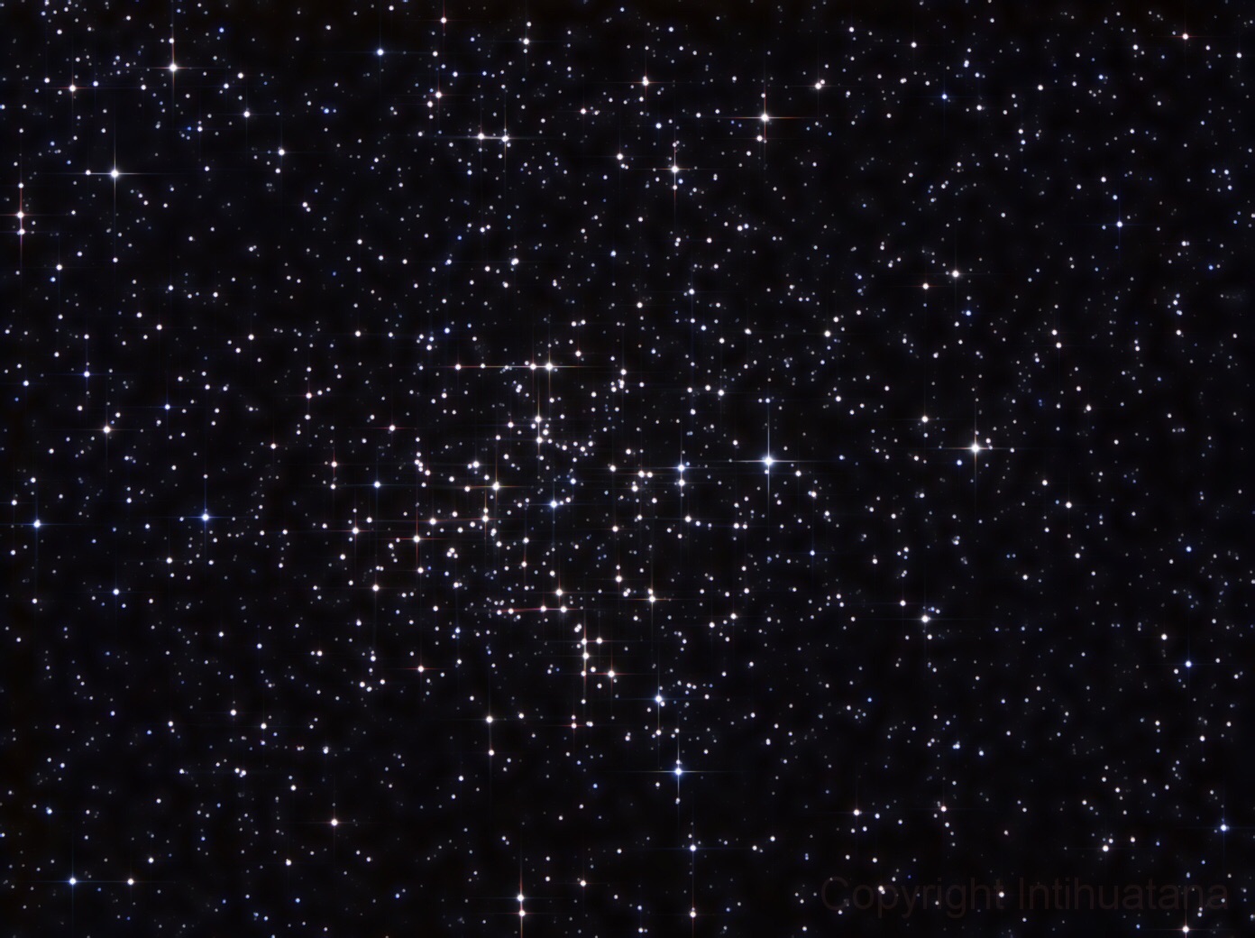
Open Cluster M38, photographed on Feb 19, 2015. Credit: Wikipedia Commons/Miguel Garcia
Perhaps by taking his time and really observing, Smyth gained some insight into the true nature of M38! Observe it yourself, and see if you can also locate NGC 1907. It’s quite a pair!
Locating Messier 38:
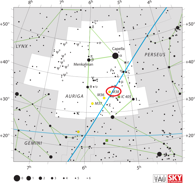
Locating Messier 38 is relatively easy once you understand the constellation of Auriga. Looking roughly like a pentagon in shape, start by identifying the brightest of these stars – Capella. Due south of it is the second brightest star which shares its border with Beta Tauri, El Nath. By aiming binoculars at El Nath, go north about 1/3 the distance between the two and enjoy all the stars!
You will note two very conspicuous clusters of stars in this area, and so did Le Gentil in 1749. Binoculars will reveal the pair in the same field, as will telescopes using lowest power. The dimmest of these is the M38, and will appear vaguely cruciform in shape. At roughly 4200 light years away, larger aperture will be needed to resolve the 100 or so fainter members. About 2 1/2 degrees to the southeast (about a finger width) you will see the much brighter M36.
More easily resolved in binoculars and small scopes, this “jewel box” galactic cluster is quite young and about 100 light years closer. If you continue roughly on the same trajectory about another 4 degrees southeast you will find open cluster M37. This galactic cluster will appear almost nebula-like to binoculars and very small telescopes – but comes to perfect resolution with larger instruments.
The location of Messier 38 open star cluster in the Auriga constellation. Credit: IAU and Sky & Telescope magazine (Roger Sinnott & Rick Fienberg)
While all three open star clusters make fine choices for moonlit or light polluted skies, remember that high sky light means less faint stars which can be resolved – robbing each cluster of some of its beauty. Messier 38 is faintest and northernmost of the trio and located almost in the center of the Auriga pentagon. Binoculars and small telescopes will easily spot its cross-shaped pattern.
And here are the quick facts on the Starfish Nebula to help you get started:
Object Name: Messier 38 Alternative Designations: M38, NGC 1912 Object Type: Galactic Open Star Cluster Constellation: Auriga Right Ascension: 05 : 28.4 (h:m) Declination: +35 : 50 (deg:m) Distance: 4.2 (kly) Visual Brightness: 7.4 (mag) Apparent Dimension: 21.0 (arc min)
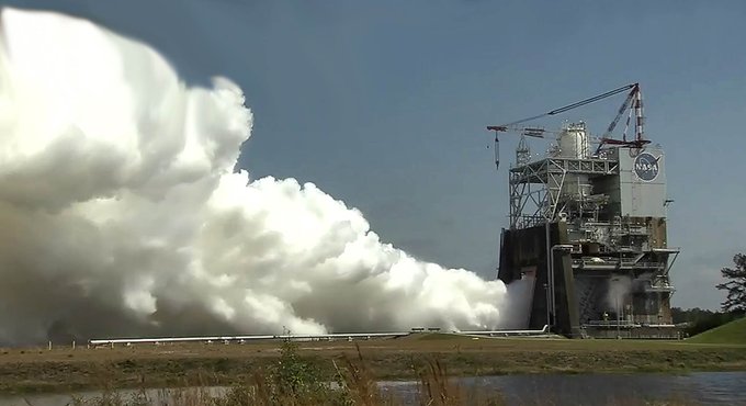
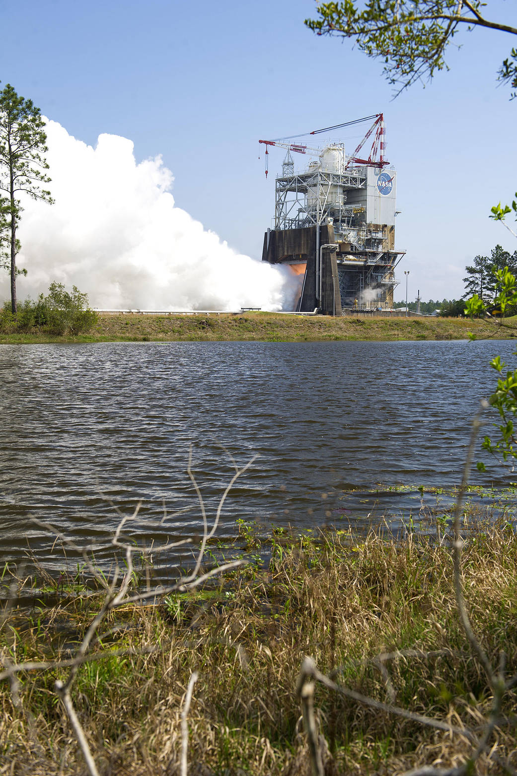
NASA engineers conduct a test of the first RS-25 engine controller that will be used on an actual Space Launch System flight on the A-2 Test Stand at Stennis Space Center on March 23, 2017. The RS-25 engine, with the flight controller, was test fired for a full-duration 500 seconds. Credits: NASA/SSC
NASA engineers conduct a test of the first RS-25 engine controller that will be used on an actual Space Launch System flight on the A-2 Test Stand at Stennis Space Center on March 23, 2017. The RS-25 engine, with the flight controller, was test fired for a full-duration 500 seconds. Credits: NASA/SSC
Engineers carried out a critical hot fire engine test firing with the first new engine controlling ‘brain’ that will command the shuttle-era liquid fueled engines powering the inaugural mission of NASA’s new Space Launch System (SLS) megarocket.
The first integrated SLS launch combining the SLS-1 rocket and Orion EM-1 deep space crew capsule could liftoff as soon as late 2018 on a mission around the Moon and back.
The full duration static fire test involved an RS-25 engine integrated with the first engine controller flight unit that will actually fly on the maiden SLS launch and took place on Thursday, March 23 at the agency’s Stennis Space Center in Bay St. Louis, Mississippi.
The 500 second-long test firing was conducted with the engine controller flight unit installed on RS-25 development engine no. 0528 on the A-2 Test Stand at Stennis.
The RS-25 engine controller is the ‘brain’ that commands the RS-25 engine and communicates between the engine and the SLS rocket. It is about the size of a dorm refrigerator.
RS-25 new engine controller. Credit: NASA/SSC
The newly developed engine controller is a modern version from the RS-25 controller that helped propel all 135 space shuttle missions to space.
“This an important – and exciting – step in our return to deep space missions,” Stennis Director Rick Gilbrech said. “With every test of flight hardware, we get closer and closer to launching humans deeper into space than we ever have traveled before.”
The modernized RS-25 engine controller was funded by NASA and created in a collaborative effort of engineers from NASA, RS-25 prime contractor Aerojet Rocketdyne of Sacramento, California, and subcontractor Honeywell of Clearwater, Florida.
“The controller manages the engine by regulating the thrust and fuel mixture ratio and monitors the engine’s health and status – much like the computer in your car,” say NASA officials.
“The controller then communicates the performance specifications programmed into the controller and monitors engine conditions to ensure they are being met, controlling such factors as propellant mixture ratio and thrust level.”
A quartet of RS-25 engines, leftover from the space shuttle era and repeatedly reused, will be installed at the base of the core stage to power the SLS at liftoff, along with a pair of extended solid rocket boosters.
The four RS-25 core stage engine will provide a combined 2 million pounds of thrust at liftoff.
In addition to being commanded by the new engine controller, the engines are being upgraded in multiple ways for SLS. For example they will operate at a higher thrust level and under different operating conditions compared to shuttle times.
To achieve the higher thrust level required, the RS-25 engines must fire at 109 percent of capability for SLS compared to operating at 104.5 percent of power level capability for shuttle flights.
The RS-25 engines “also will operate with colder liquid oxygen and engine compartment temperatures, higher propellant pressure and greater exhaust nozzle heating.”
SLS will be the world’s most powerful rocket and send astronauts on journeys into deep space, further than human have ever travelled before.
For SLS-1 the mammoth booster will launch in its initial 70-metric-ton (77-ton) Block 1 configuration with a liftoff thrust of 8.4 million pounds – more powerful than NASA’s Saturn V moon landing rocket.
NASA engineers conduct a test of the first RS-25 engine controller that will be used on an actual Space Launch System flight on the A-2 Test Stand at Stennis Space Center on March 23, 2017. The RS-25 engine, with the flight controller, was test fired for a full-duration 500 seconds. Credits: NASA/SSC
The next step is evaluating the engine firing test results, confirming that all test objectives were met and certifying that the engine controller can be removed from the RS-25 development engine and then be installed on one of four flight engines that will help power SLS-1.
During 2017, two additional engine controllers for SLS-1 will be tested on the same development engine at Stennis and then be installed on flight engines after certification.
Finally, “the fourth controller will be tested when NASA tests the entire core stage during a “green run” on the B-2 Test Stand at Stennis. That testing will involve installing the core stage on the stand and firing its four RS-25 flight engines simultaneously, as during a mission launch,” says NASA.
Numerous RS-25 engine tests have been conducted at Stennis over more than 4 decades to certify them as flight worthy for the human rated shuttle and SLS rockets.
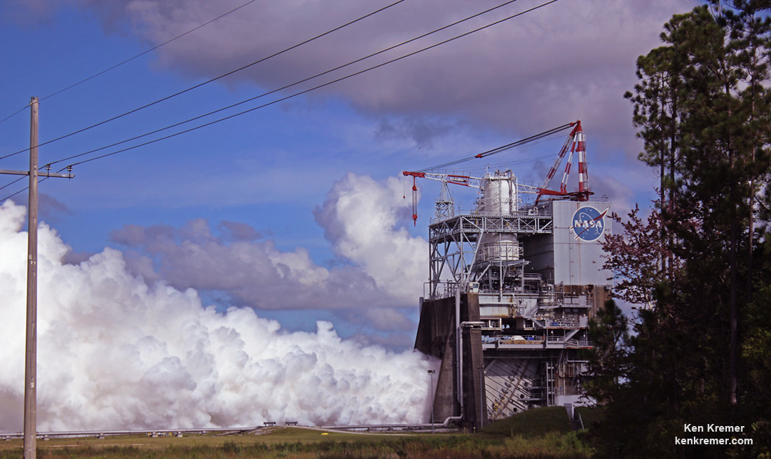
NASA engineers successfully conducted a development test of the RS-25 rocket engine Thursday, Aug. 18, 2016 at NASA’s Stennis Space Center near Bay St. Louis, Miss. The RS-25 will help power the core stage of the agency’s new Space Launch System (SLS) rocket for the journey to Mars. Credit: Ken Kremer/kenkremer.com
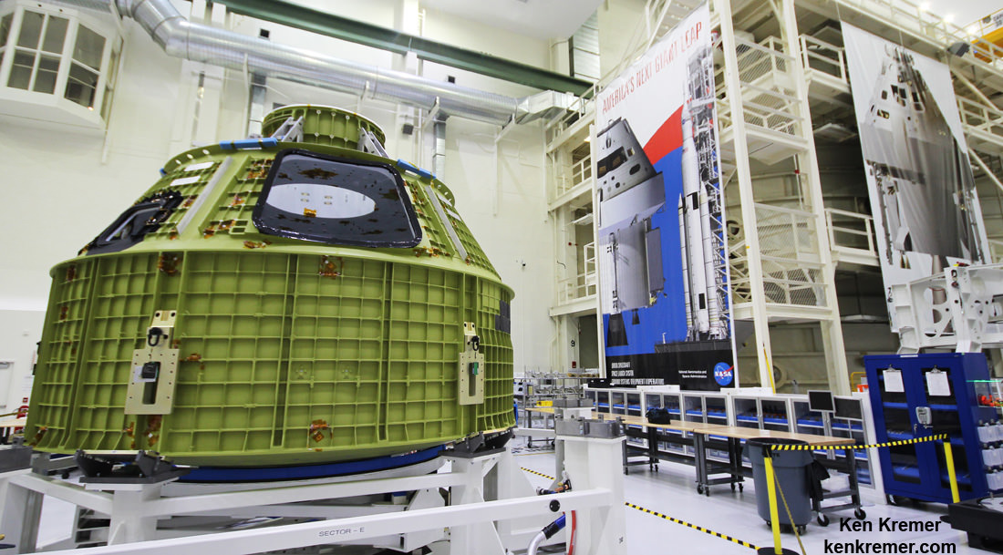
Although NASA is still targeting SLS-1 for launch in Fall 2018 on an uncrewed mission, the agency is currently conducting a high level evaluation to determine whether the Orion EM-1 capsule can be upgraded in time to instead fly a human crewed mission with two astronauts before the end of 2019 – as I reported here.
The Orion EM-1 capsule is currently being manufactured at the Neil Armstrong Operations and Checkout Building at the Kennedy Space Center by prime contractor Lockheed Martin.
Orion crew module pressure vessel for NASA’s Exploration Mission-1 (EM-1) is unveiled for the first time on Feb. 3, 2016 after arrival at the agency’s Kennedy Space Center (KSC) in Florida. It is secured for processing in a test stand called the birdcage in the high bay inside the Neil Armstrong Operations and Checkout (O&C) Building at KSC. Launch to the Moon is slated in 2018 atop the SLS rocket. Credit: Ken Kremer/kenkremer.com
Stay tuned here for Ken’s continuing Earth and Planetary science and human spaceflight news.
Aerojet Rocketdyne technicians inspect the engine controller that will be used for the first integrated flight of NASA’s Space Launch System and Orion in late 2018. The engine controller was installed on RS-25 development engine no. 0528 for testing at Stennis Space Center on the A-2 Test Stand on March 23, 2017. The RS-25 engine, with the flight controller, was test fired for a full-duration 500 seconds. Credits: NASA/SSC
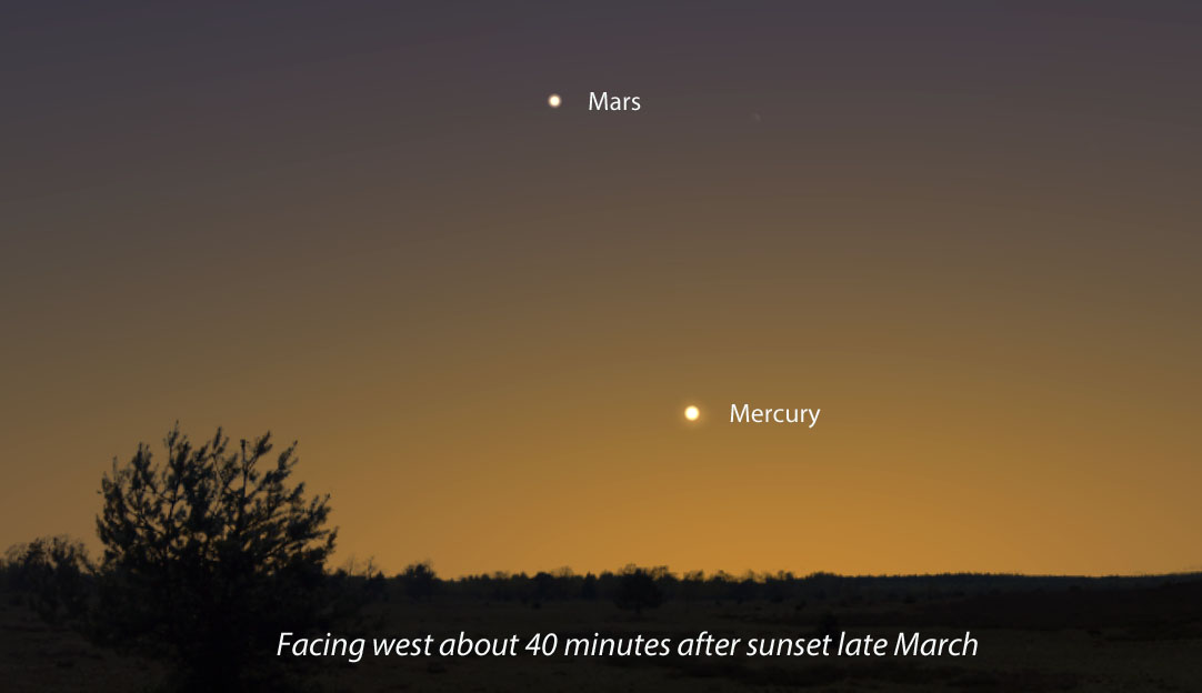
Mercury requests the company of your gaze now through the beginning of April, when it shines near Mars low in the west after sunset. Created with Stellarium
March has been a busy month for planet and comet watchers. Lots of action. Venus, the planet that’s captured our attention at dusk in the west for months, is in inferior conjunction with the Sun today. Watch for it to rise before the Sun in the eastern sky at dawn in about a week.
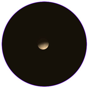
Mercury like Venus and the Moon shows phases when viewed through a telescope. Right now, the planet is in waning gibbous phase. Stellarium
As Venus flees the evening scene, steadfast Mars and a new planet, Mercury keep things lively. For northern hemisphere skywatchers, this is Mercury’s best dusk apparition of the year. If you’d like to make its acquaintance, this week and next are best. And it’s so easy! Just find a spot with a wide open view of the western horizon, bring a pair of binoculars for backup and wait for a clear evening.
Plan to watch starting about 40 minutes after sundown. From most locations, Mercury will appear about 10° or one fist held at arm’s length above the horizon a little bit north of due west. Shining around magnitude +0, it will be the only “star” in that part of the sky. Mars is nearby but much fainter at magnitude +1.5. You’ll have to wait at least an hour after sunset to spot it.
Have a telescope? Check out the planet using a magnification around 50x or higher. You’ll see that it looks like a Mini-Me version of the Moon. Mercury is brightest when closest to full. Over the next few weeks, it will wane to a crescent while increasing in apparent size.
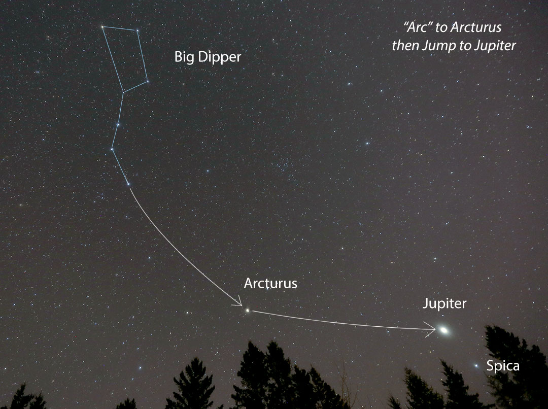
If you have any difficulty finding brilliant Jupiter and its current pal, Spica, just start with the Big Dipper, now high in the northeastern sky at nightfall. Use the Dipper’s handle to “arc to Arcturus” and then “jump to Jupiter.” Credit: Bob King
If you like planets, don’t forget the combo of Jupiter and Spica at the opposite end of the sky. Jupiter climbs out of bed and over the southeastern horizon about 9 p.m. local time in late March, but to see it and Spica, Virgo’s brightest star, give it an hour and look again at 10 p.m. or later. Quite the duo!
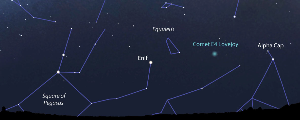
You’re not afraid of getting up with the first robins are you? If you set your alarm to a half hour or so before the first hint of dawn’s light and find a location with an open view of the southeastern horizon, you might be first in your neighborhood to spot Terry Lovejoy’s brand new comet. His sixth, the Australian amateur discovered C/2017 E4 Lovejoyon the morning of March 10th in the constellation Sagittarius at about 12th magnitude.
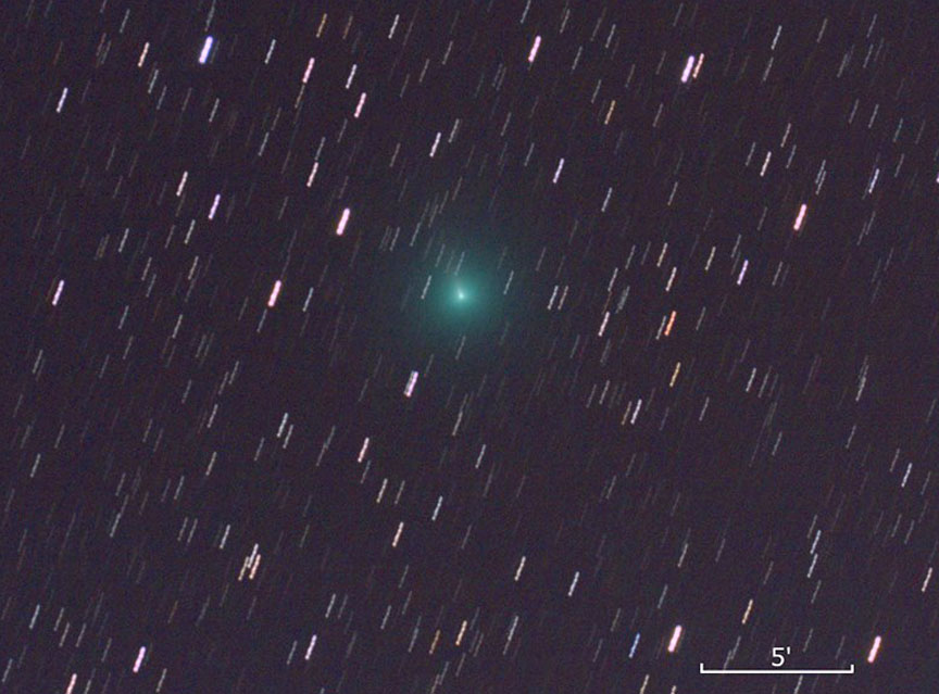
C/2017 E4 Lovejoy glows blue-green this morning March 26. Structure around the nucleus including a small jet is visible. The comet is currently in Aquarius and quickly moving north and will reach perihelion on April 23. Credit: Terry Lovejoy
The comet has rapidly brightened since then and is now a small, moderately condensed fuzzball of magnitude +9, bright enough to spot in a 6-inch or larger telescope. Some observers have even picked it up in large binoculars. Lovejoy’s comet should brighten by at least another magnitude in the coming weeks, putting it within 10 x 50 binocular range.
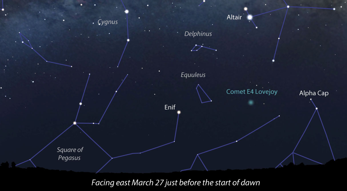
This map shows the sky tomorrow morning before dawn from the central U.S. (latitude about 41° north). Created with Stellarium
Good news. E4 Lovejoy is moving north rapidly and is now visible about a dozen degrees high in Aquarius just before the start of dawn. I’ll be out the next clear morning, eyepiece to eye, to welcome this new fuzzball from beyond Neptune to my front yard. The map above shows the eastern sky near dawn and a general location of the comet. Use the more detailed map below to pinpoint it in your binoculars and telescope.
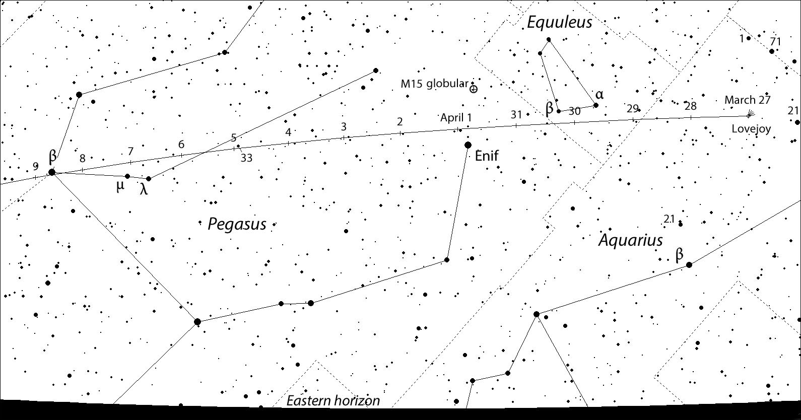
This chart shows the comet’s position nightly (5:30 a.m. CDT) through April 9. On the morning of April 1 it passes just a few degrees below the bright globular cluster M15. Click to enlarge, save and then print out for use at the telescope. Map: Bob King, Source: Chris Marriott’s SkyMap
Spring brings with it a new spirit and the opportunity to get out at night free of the bite of mosquitos or cold. Clear skies!
As you probably know, NASA recently announced plans to send a mission to Jupiter’s moon Europa. If all goes well, the Europa Clipper will blast off for the world in the 2020s, and orbit the icy moon to discover all its secrets.
And that’s great and all, I like Europa just fine. But you know where I’d really like us to go next? Titan.
Titan, as you probably know, is the largest moon orbiting Saturn. In fact, it’s the second largest moon in the Solar System after Jupiter’s Ganymede. It measures 5,190 kilometers across, almost half the diameter of the Earth. This place is big.
It orbits Saturn every 15 hours and 22 days, and like many large moons in the Solar System, it’s tidally locked to its planet, always showing Saturn one side.
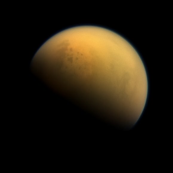
Titan image taken by Cassini on Oct. 7, 2013 (Credit: NASA/JPL-Caltech/Space Science Institute)
Before NASA’s Voyager spacecraft arrived in 1980, astronomers actually thought that Titan was the biggest moon in the Solar System. But Voyager showed that it actually has a thick atmosphere, that extends well into space, making the true size of the moon hard to judge.
This atmosphere is one of the most interesting features of Titan. In fact, it’s the only moon in the entire Solar System with a significant atmosphere. If you could stand on the surface, you would experience about 1.45 times the atmospheric pressure on Earth. In other words, you wouldn’t need a pressure suit to wander around the surface of Titan.
You would, however, need a coat. Titan is incredibly cold, with an average temperature of almost -180 Celsius. For you Fahrenheit people that’s -292 F. The coldest ground temperature ever measured on Earth is almost -90 C, so way way colder.
You would also need some way to breathe, since Titan’s atmosphere is almost entirely nitrogen, with trace amounts of methane and hydrogen. It’s thick and poisonous, but not murderous, like Venus.
Titan has only been explored a couple of times, and we’ve actually only landed on it once.
The first spacecraft to visit Titan was NASA’s Pioneer 11, which flew past Saturn and its moons in 1979. This flyby was followed by NASA’s Voyager 1 in 1980 and then Voyager 2 in 1981. Voyager 1 was given a special trajectory that would take it as close as possible to Titan to give us a close up view of the world.
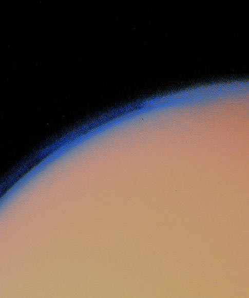
Saturn’s moon Titan lies under a thick blanket of orange haze in this Voyager 1 picture. Credit: NASA
Voyager was able to measure its atmosphere, and helped scientists calculate Titan’s size and mass. It also got a hint of darker regions which would later turn out to be oceans of liquid hydrocarbons.
The true age of Titan exploration began with NASA’s Cassini spacecraft, which arrived at Saturn on July 4, 2004. Cassini made its first flyby of Titan on October 26, 2004, getting to within 1,200 kilometers or 750 miles of the planet. But this was just the beginning. By the end of its mission later this year, Cassini will have made 125 flybys of Titan, mapping the world in incredible detail.
Cassini saw that Titan actually has a very complicated hydrological system, but instead of liquid water, it has weather of hydrocarbons. The skies are dotted with methane clouds, which can rain and fill oceans of nearly pure methane.
And we know all about this because of Cassini’s Huygen’s lander, which detached from the spacecraft and landed on the surface of Titan on January 14, 2005. Here’s an amazing timelapse that shows the view from Huygens as it passed down through the atmosphere of Titan, and landed on its surface.
Huygens landed on a flat plain, surrounded by “rocks”, frozen globules of water ice. This was lucky, but the probe was also built to float if it happened to land on liquid instead.
It lasted for about 90 minutes on the surface of Titan, sending data back to Earth before it went dark, wrapping up the most distant landing humanity has ever accomplished in the Solar System.
Although we know quite a bit about Titan, there are still so many mysteries. The first big one is the cycle of liquid. Across Titan there are these vast oceans of liquid methane, which evaporate to create methane clouds. These rain, creating mists and even rivers.
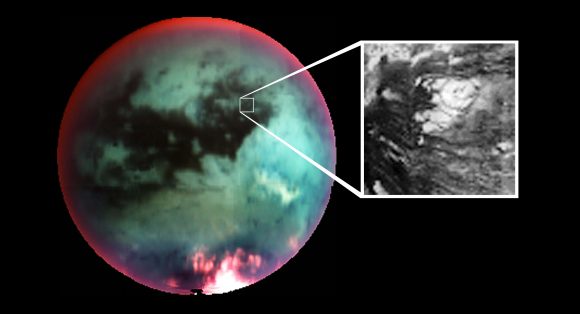
This false-color mosaic of Saturn’s largest moon Titan, obtained by Cassini’s visual and infrared mapping spectrometer, shows what scientists interpret as an icy volcano. Credit: NASA/JPL/University of Arizona
Is it volcanic? There are regions of Titan that definitely look like there have been volcanoes recently. Maybe they’re cryovolcanoes, where the tidal interactions with Saturn cause water to well up from beneath crust and erupt onto the surface.
Is there life there? This is perhaps the most intriguing possibility of all. The methane rich system has the precursor chemicals that life on Earth probably used to get started billions of years ago. There’s probably heated regions beneath the surface and liquid water which could sustain life. But there could also be life as we don’t understand it, using methane and ammonia as a solvent instead of water.
To get a better answer to these questions, we’ve got to return to Titan. We’ve got to land, rove around, sail the oceans and swim beneath their waves.
Now you know all about this history of the exploration of Titan. It’s time to look at serious ideas for returning to Titan and exploring it again, especially its oceans.
Planetary scientists have been excited about the exploration of Titan for a while now, and a few preliminary proposals have been suggested, to study the moon from the air, the land, and the seas.
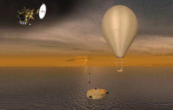
The spacecraft, balloon, and lander of the Titan Saturn System Mission. Credit: NASA Jet Propulsion Laboratory
First up, there’s the Titan Saturn System Mission, a mission proposed in 2009, for a late 2020s arrival at Titan. This spacecraft would consist of a lander and a balloon that would float about in the atmosphere, and study the world from above. Over the course of its mission, the balloon would circumnavigate Titan once from an altitude of 10km, taking incredibly high resolution images. The lander would touch down in one of Titan’s oceans and float about on top of the liquid methane, sampling its chemicals.
As we stand right now, this mission is in the preliminary stages, and may never launch.
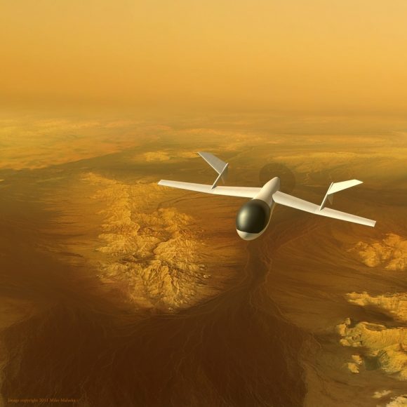
The Aerial Vehicle for In-situ and Airborne Titan Reconnaissance (AVIATR) concept for an aerial explorer for Titan. Credit: Mike Malaska
In 2012, Dr. Jason Barnes and his team from the University of Idaho proposed sending a robotic aircraft to Titan, which would fly around in the atmosphere photographing its surface. Titan is actually one of the best places in the entire Solar System to fly an airplane. It has a thicker atmosphere and lower gravity, and unlike the balloon concept, an airplane is free to go wherever it needs powered by a radioactive thermal generator.
Although the mission would only cost about $750 million or so, NASA hasn’t pushed it beyond the conceptual stage yet.
On the left is TALISE (Titan Lake In-situ Sampling Propelled Explorer), the ESA proposal. This would have it’s own propulsion, in the form of paddlewheels. Credit: bisbos.com
An even cooler plan would put a boat down in one of Titan’s oceans. In 2012, a team of Spanish engineers presented their idea for how a Titan boat would work, using propellers to put-put about across Titan’s seas. They called their mission the Titan Lake In-Situ Sampling Propelled Explorer, or TALISE.
Propellers are fine, but it turns out you could even have a sailboat on Titan. The methane seas have much less density and viscosity than water, which means that you’d only experience about 26% the friction of Earth. Cassini measured windspeeds of about 3.3 m/s across Titan, which half the average windspeed of Earth. But this would be plenty of wind to power a sail when you consider Titan’s thicker atmosphere.
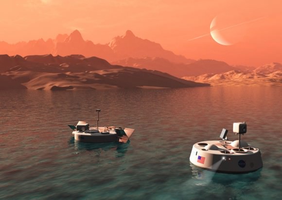
And here’s my favorite idea. A submarine. This 6-meter vessel would float on Titan’s Kraken Mare sea, studying the chemistry of the oceans, measuring currents and tides, and mapping out the sea floor.
It would be capable of diving down beneath the waves for periods, studying interesting regions up close, and then returning to the surface to communicate its findings back to Earth. This mission is in the conceptual stage right now, but it was recently chosen by NASA’s Innovative Advanced Concepts Group for further study. If all goes well, the submarine would travel to Titan by 2038 when there’s a good planetary alignment.
Okay? Are you convinced? Let’s go back to Titan. Let’s explore it from the air, crawl around on the surface and dive beneath its waves. It’s one of the most interesting places in the entire Solar System, and we’ve only scratched the surface.
If I’ve done my job right, you’re as excited about a mission to Titan as I am. Let’s go back, let’s sail and submarine around that place. Let me know your thoughts in the comments.